article

1 Overview

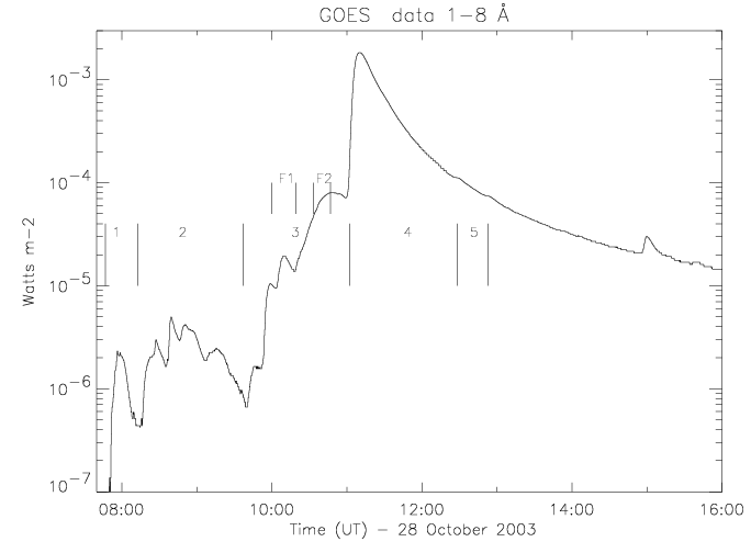
Figure 1: Time evolution of the GOES X-ray fluxes. Here we focus on the October 28, 2003 X17 flare. In the bottom plot, the timings of the 5 successive CDS rasters are indicated. CDS observed the two precursor M-class flares F1 and F2 with the third raster.

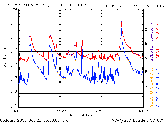
2 The two pre-events, M-class flares

SOHO CDS observed with the 3rd raster during 09:37-11:02 UT. CDS observed two distinct M-class flares, with strong Fe XIX emission (saturated in the two cores). The first one (F1) was observed during 10:00-10:19 UT, while the second (F2) during 10:33-10:47 UT. The first flare was also observed by TRACE.

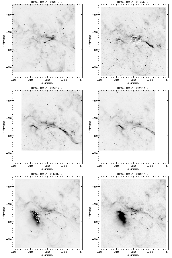
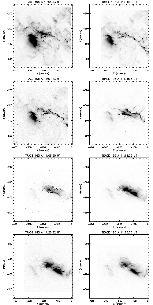
Figure 2: Sequence of TRACE 195 Å images, showing the two M-class flares. Between 10:24 and 10:49 UT TRACE did not observe. Note the contours of Fe XIX emission of the two flares observed by CDS.

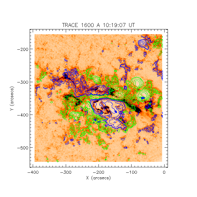
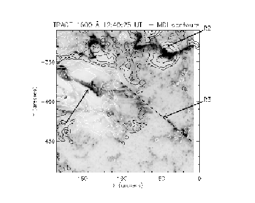
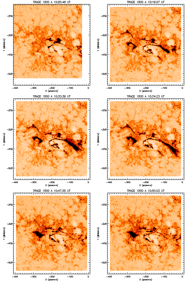
Figure 3: Sequence of TRACE 1600 Å images, showing the two M-class flares. Between 10:24 and 10:49 UT TRACE did not observe.

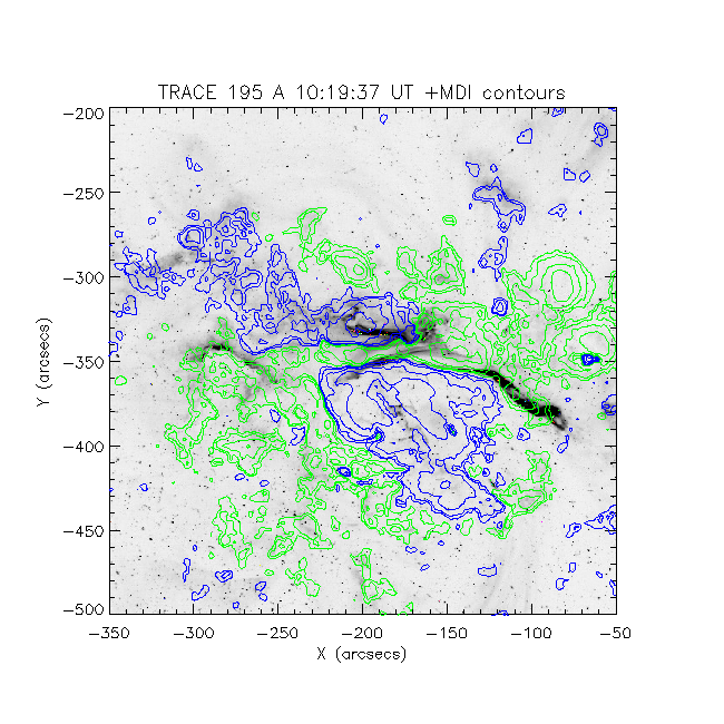
Figure 4: TRACE 195,1600 Å with contours from SOHO/MDI magnetogram. The M-class flare occurred in the region of mixed polarity. Note also the filament eruption associated with this flare.

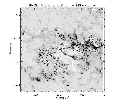
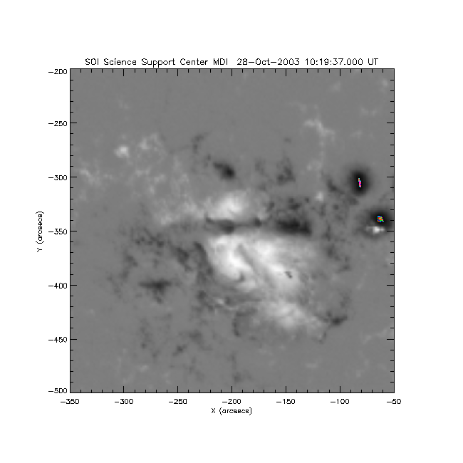
Figure 5: SOHO/MDI magnetogram.

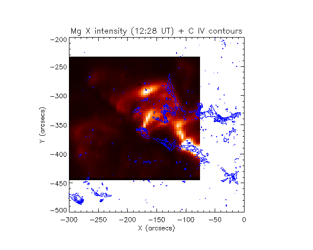
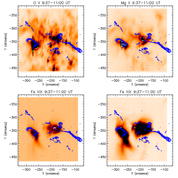
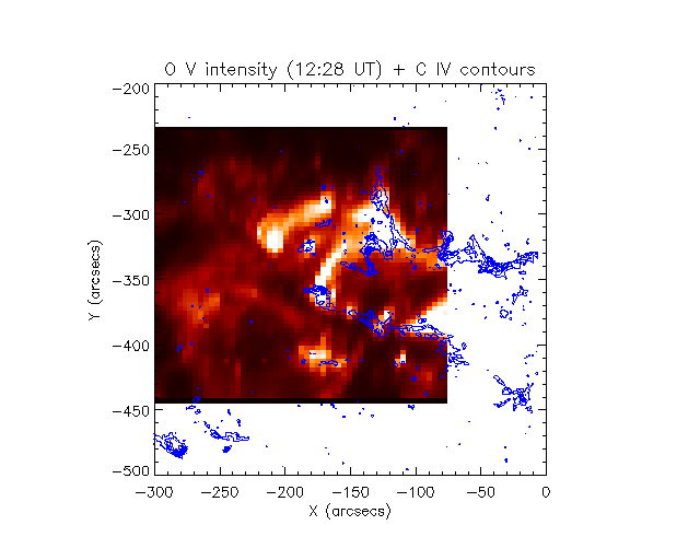
Figure 6: CDS monochromatic images at transition region (O V), coronal (Mg X) and flare (Fe XIX) temperatures, during the long CDS scan which observed the two F1,F2 M-class flares. Overlaid are contours of TRACE 1600 Å. Notice the complex structure of the second flare (left) in the enhanced Fe XIX image.

3 The X17 flare

Figure 7: Sequence of TRACE 195 Å images during the X17 flare. The first three images are shown with a different intensity scale, compared to the following ones.

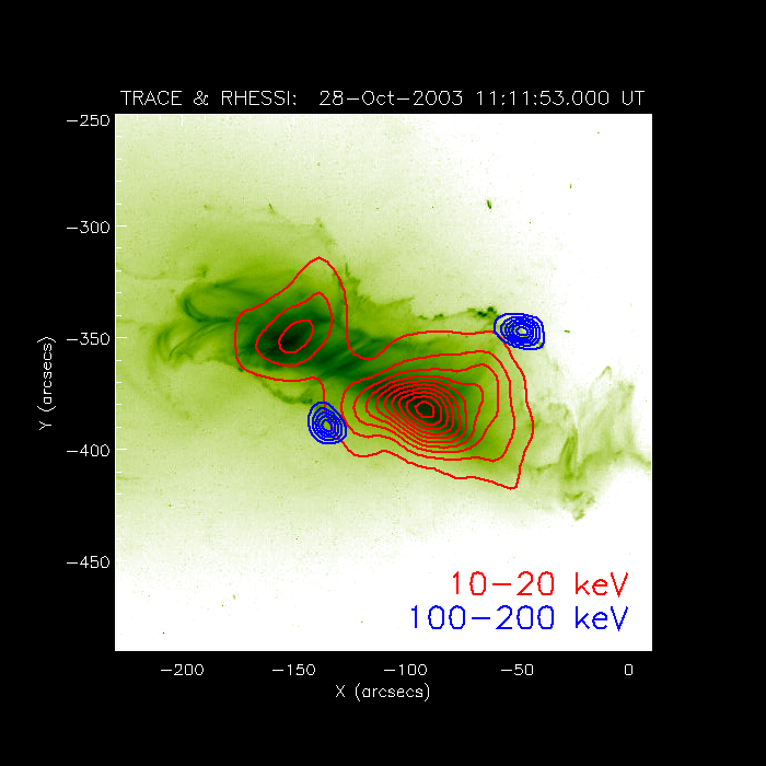
Figure 8: TRACE + RHESSI (from Sam Krucker)

SOHO/EIT 195 A movie

SOHO/LASCO movie

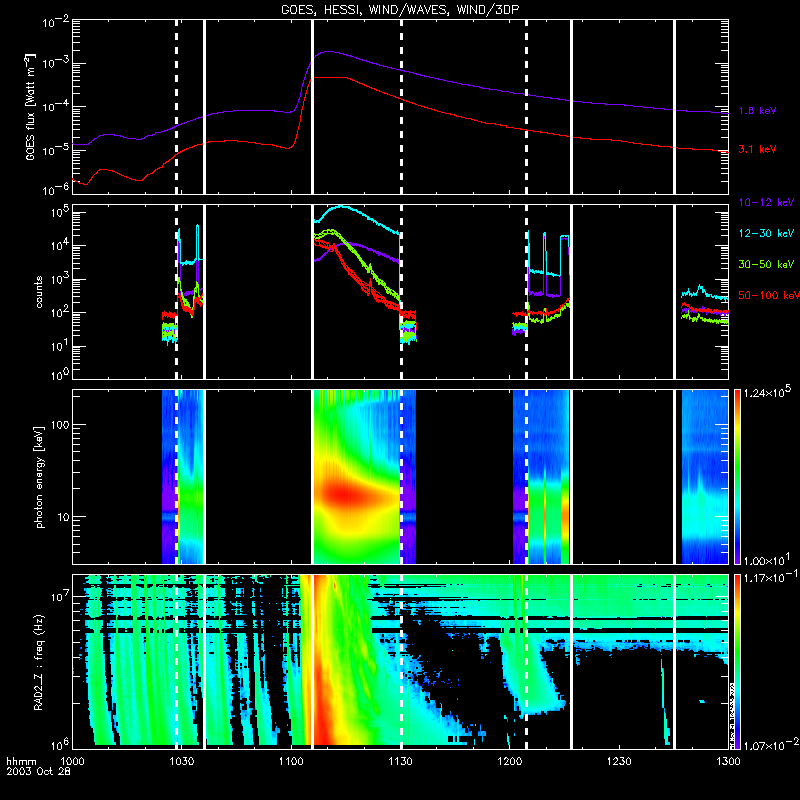
Figure 9: GOES + RHESSI + ...

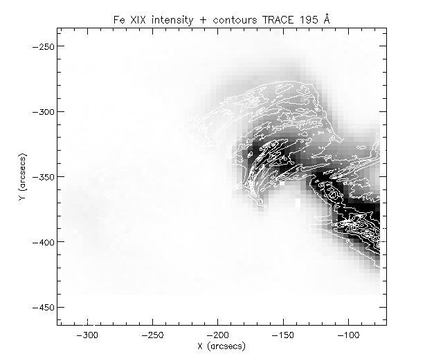
Post-flare arcade

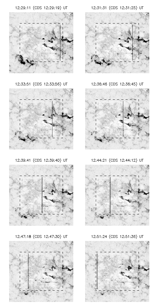
Here we show results concerning the 5th CDS observation (12:28-12:52 UT). During this time, TRACE 195 and 1600 Å images show that the 2-ribbon structure and the arcade of loops is approximately stationary, with some apparent flows along the loops.

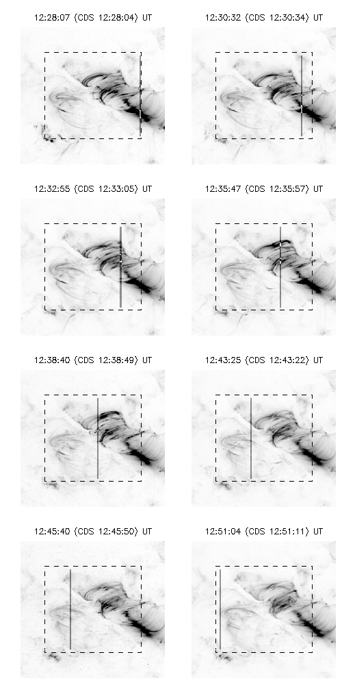
Figure 10: Sequence of TRACE 195, 1600 Å images during the CDS raster, shown with the same intensity scale. The FOV of the CDS raster, and the position of the slit. Notice that overall the loop structures seen in TRACE 195 Å and the ribbon structures seen in TRACE 1600 Å remain largely unchanged.

195 A movie

1600 A movie

halpha

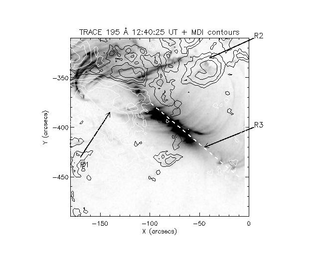
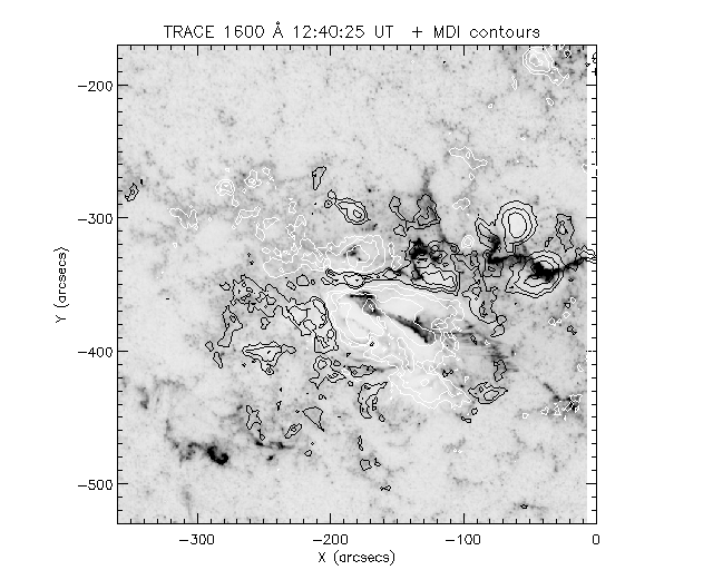
Figure 11: TRACE 195, 1600 Å images, with contours from the SOHO/MDI magnetogram (200, 500, 1000 G). Notice the arcade of loops seen in TRACE 195 Å connecting the ribbon structures R1, R2 which are located above the sunspot regions of opposite polarity. Also note the system of loops in TRACE 195 Å which connects the ribbon R3 to R1 and R2. The ribbon R3 is seen in TRACE 1600 Å as an almost straight line of emission. Flows in TRACE 1600 Å from R3 to R1 are seen. The cantral part of R3 is also the loaction of the strongest emission in TRACE 195 Å.

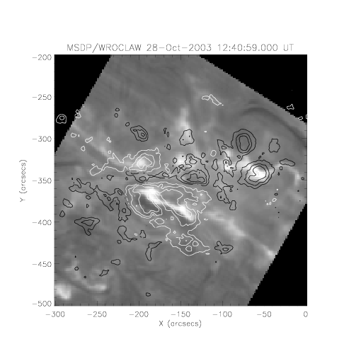
Figure 12: Ha observation from Bialkov, with contours of SOHO/MDI magnetograms. Note the similarity with the TRACE 1600 Å image and the presence of the three ribbon structures.

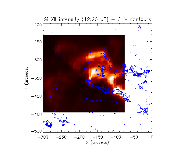
Figure 13: CDS intensity maps with contours of TRACE 1600 (showing the ribbons). The post-flare loops show emission at all temperatures

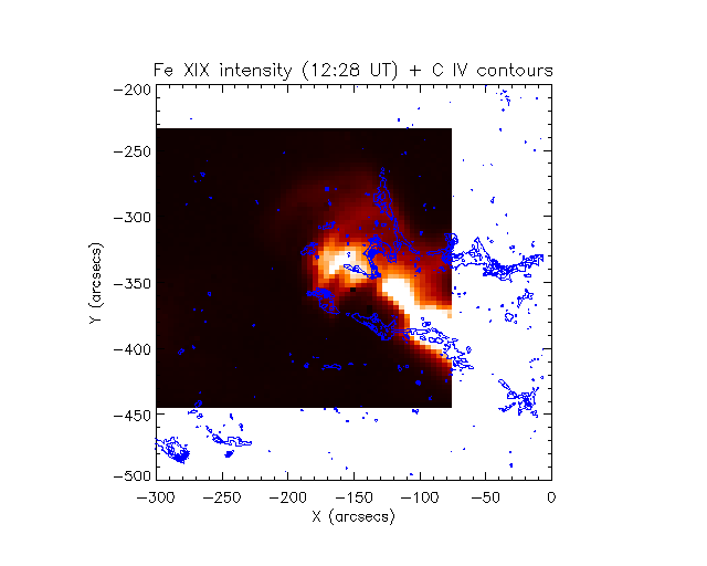
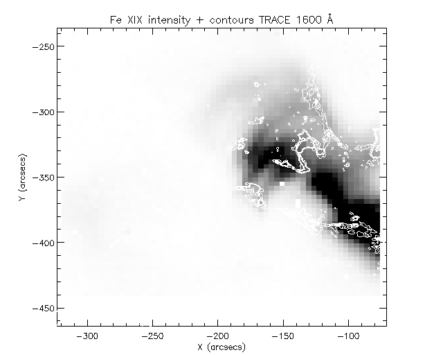
Figure 14: intensity in Fe XIX with contours of TRACE 1600,195 Å intensities.

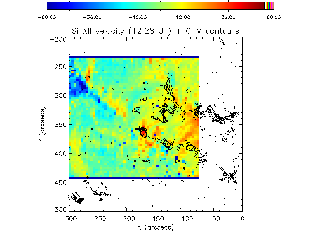
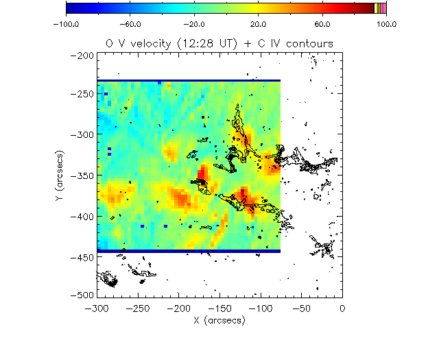
Figure 15: CDS velocity map in the transition region (O V) with contours of TRACE 1600 (showing the ribbons). Strong downflows (v @ 50-100 km/s ) in the ribbons are observed.

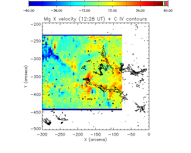
Figure 16: CDS velocity maps in coronal lines with contours of TRACE 1600 (showing the ribbons). Strong downflows (v @ 50-100 km/s ) in the ribbons are observed.

The X17 flare presented great complexity. We have used the CDS to understand the temperature structure of the various events.

Two precursor M-class events have been observed with CDS. The first one was also observed by TRACE, while the second, more important one, was not observed by TRACE. The second one had a complex structure of hot loops.

During the precursor events the filament becomes activated.

During the X17 flare the ribbons quickly separate and an arcade system of loops forms. These loops are multi-thermal, with the hottest part in the central region.

Strong downflows (v @ 50-100 km/s ), in particular at transition region temperatures are observed in the ribbons.

File translated from T_EX by T_TH, version 3.08.
On 17 May 2005, 10:45.