|
| SOHO CDS Guide |
| Instrument, calibration, data analysis |
| All you did not want to know about CDS... |
| ... and some spectroscopic diagnostics |
| Giulio Del Zanna (G.Del-Zanna@damtp.cam.ac.uk) |
| Medoc 2003 TOSTISP workshop |
This material is virtually a merged version of my PhD thesis, the CDS user guide at RAL and the CDS user guide at MSSL, plus various material that I have produced and is available on the WWW (e.g. CHIANTI user guides).
Note that some material is not published.
RAL   (UK)

CDS main WWW pages:

http://solg2.bnsc.rl.ac.uk/


Principle Investigator:        Andrzej Fludra
             (Richard Harrisons until Sept 2003)

Project Scientist:             Peter Young
Science Operations Manager:    David Pike
Instrument Operations Manager: Jeff Payne
Science Software:   David Pike
                    William Thompson
                    Dominic Zarro

(a lot of useful software was developed at Oslo
by Stein Vidar Haugan and others)


MSSL (UK)

Solar UK Research Facility  (Carl Foley)

http://surfwww.mssl.ucl.ac.uk/surf/

Giulio Del Zanna Phd Thesis and CDS WWW pages:

http://www.damtp.cam.ac.uk/user/astro/gd232/astro.html
Read CDS Software Notes. An enormous amount of information.
Sign up to the CDS Software and Data Analysis Discussion List
Read IDL procedures headers
Get involved !
Be open-minded and do not take any results for granted.
Do not be discouraged by the complexities, for the CDS data have a great diagnostic potential !
|
|
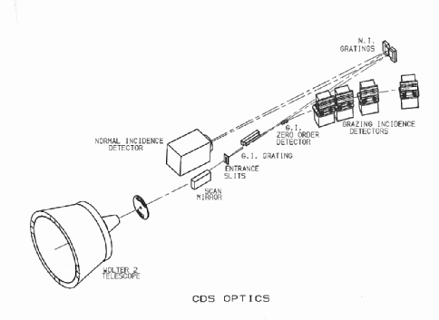
The CDS instrument (Figure 1) consists of a Wolter-Schwartzschild type II grazing incidence telescope, a scan mirror, a set of different slits, and two spectrometers that do not observe simultaneously, the normal incidence spectrometer (NIS) and the grazing incidence spectrometer (GIS).
The slits provide various fields of view (2óó×2óó, 4óó×4óó, 2óó×240óó, 4óó×240óó, 90óó×240óó, 8óó×50óó) and are normally oriented along the solar N-S direction.
Any position on the Sun is commonly indicated by two coordinates, Solar X and Solar Y, also used to indicate the centres of the pointing of any CDS observation. Solar X is given in arc sec from the disc centre along the East-West (E-W) direction, while Solar Y indicates arc sec from the disc centre along the South-North (S-N) direction. Note that 1óó corresponds on the Sun to 700 km.
The internal scan mirror and slit movement of CDS allow CDS rasters to cover a maximum area of 4' square within a single raster. The E-W coverage is created by the scan mirror which can move in steps of 2.03" (normally assumed to be 2"). Movement can only be in one direction from West to East.
In NIS the N-S coverage is usually provided by the long slit (normal slits are 2"x240" or 4"x240").
For GIS the N-S dimension is scanned by moving one of the small square slits which can move in steps of 1.01" (normally assumed to be 1"!).
The pointing to any location is accomplished through two mechanisms, one external and one internal.
The first is achieved with the use of external legs, that move the whole CDS instrument at 45 degrees to the N-S and E-W directions, with about 2óó steps. The overall pointing accuracy of the CDS instrument has been at best 10óó. The area reachable can extend out to a maximum 1.4 solar radii in certain directions.
The internal movement is more accurate because it is done via the movement of the scan mirror and the slits, with 2óó steps, and has a negligible error. It is limited to 4' in either direction.
The solar rotation produces an apparent movement of any feature of about 10óó in an hour at the sun centre. Considering that the typical duration of a CDS observation is one hour, rastering over a region of the order of one arc min, the solar rotation is often a non-negligible effect in observations near sun-centre, and is further complicated by the differential rotation of the solar corona.
CDS has feature tracking software, which moves the entire instrument, but since the accuracy of the movements is much less than the spatial resolution, it is not generally recommended.
CDS software note #45 details the limitations, but in short these are:
1) The minimum E-W movement is approximately 2óó.
2) the actual movement may often be 2óó ▒2óó with the result that the effect may be `worse than doing nothing', depending on what effect was intended.
3) The default interval for updating the pointing is 600 seconds. If an individual raster duration is less than this, no correction will ever occur.
The NIS is composed of two normal incidence gratings that disperse the light into the NIS detector, known as the viewfinder detector subsystem, or VDS. The gratings are slightly tilted, in order to produce two wave-bands (NIS 1: 308 - 379 Å and NIS 2: 513 - 633 Å;) on the same detector, one on top of the other (see Figure 3.6.1). The spectral resolution is @ 0.35 Å for NIS 1 and @ 0.5 Å for NIS 2. Second order lines have been observed only in NIS 2.
The NIS can provide monochromatic images of the solar field of view. This is accomplished with the rastering of a region, moving a mirror and producing contiguous images of one of the long slits. The rastering is performed from west to east (being the normal alignment of CDS with the slits in the solar N-S direction).
Telemetry constraints usually make it necessary to pre-select a number of NIS wavelength windows to be extracted on-board from the spectra, before the data are telemetered to the ground.
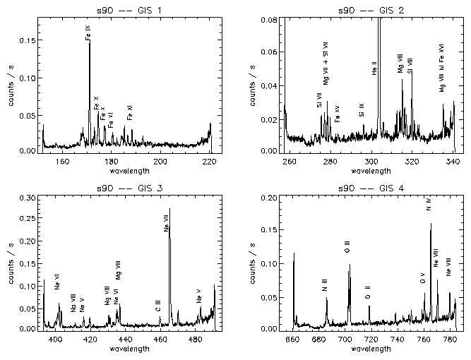
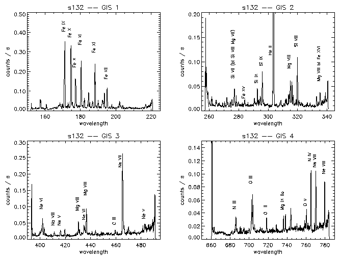
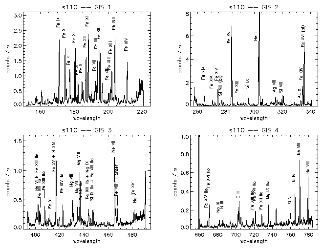
The grazing incidence spectrometer (GIS) has a grazing incidence spherical grating that disperses the incident light to four microchannel plate (MCP) detectors placed along the Rowland Circle (GIS 1: 151 - 221 Å, GIS 2: 256 - 341 Å, GIS 3: 393 - 492 Å and GIS 4: 659 - 785 Å;).
The spectral resolution of the GIS detectors is about 0.5 Å. Many second order lines have been observed in GIS 3 and GIS 4.
The GIS is astigmatic, focusing the image of the slit along the direction of dispersion but not perpendicular to it.
Images of the Sun are obtained using a pinhole slit and combining movements of the slit and of the scan mirror.
Normally, the movements are such that an area of the Sun is rastered in a zig-zag pattern, starting from south to north and from west to east (in normal CDS alignment).
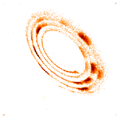
The GIS detectors are composed of a stack of micro-channel plates (MCPs), and a spiral anode (SPAN) to read the position and charge of the electron cloud created by the MCPs. The reading is converted with an 8-bit analogue to digital converter (ADC) which outputs data at (x, y) position values (known as GIS raw data). The (x, y) values form a spiral in cartesian coordinates (see Figure 2), which contains all the one-dimensional spectral information (the GIS being astigmatic, no more information is needed). The wavelength varies with distance along the spiral and the width of each arm is related to the noise in the electronics.
|
A set of parameters, called a look up table (LUT) is produced for each detector, fitting this spiral pattern, in order to convert the signal produced by the photon events to an array of 2048 spectral data points as a function of wavelength.
Because the gain in the micro channel plates is sensitive to the intensity, the voltages applied to each detector are adjusted depending on the slit used and the solar conditions (active or quiet sun), creating different spiral patterns, each requiring a different set of LUTs.
Because it takes too long to telemeter to the ground the raw data, this is done only once in a while to generate the LUTs. Normally the raw data are converted on-board by applying a set of LUTs, uniquely identified by a number GSET_ID, to the raw data. Various sets of LUTs are stored on-board for use, and loaded before the GIS starts exposing (it takes about half an hour). It is important, during planning, to select the correct set of LUTs (i.e. GSET_ID number) for the type of observation, otherwise the telemetered spectra are not usable.
The GIS spectra have various effects that must be carefully considered before starting any data analysis. Some effects are typical of any MCP detector, and are
electronic dead times
short term gain depression
long term gain depression.
The GIS operates by sending a continuous stream of event positions to the Command and Data-Handling System (CDHS). The various electronic dead-times are such that any events occurring within about 10 ms of each other will be rejected, and higher rates will render the data meaningless.
Short term gain depression occurs when count rates per pixel are above 40. In this situation, the MCP cannot re-charge fast enough to provide full gain for every event, and the data are not usable.
Long term gain depression is an ageing effect, a reduction in detector sensitivity over a long time interval due to continued illumination. The applied high voltage can be increased to compensate for the decrease in the MCP gain with time. However, the gain depression will be greatest at the position of the brightest lines so a wavelength-dependent effect will remain.
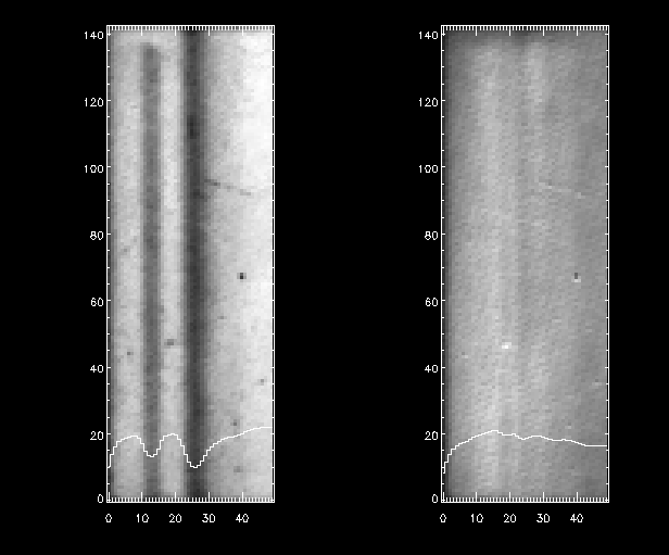
The profiles of the GIS lines are predominantly instrumental. They are corrupted by the superposition of a spiky effect on the whole spectrum, referred to as fixed patterning. Counts falling near the boundary of a pixel can be shifted to neighbouring pixels, producing narrow spikes and troughs in the profiles of the emission lines. Weaker lines can appear swamped by this effect.
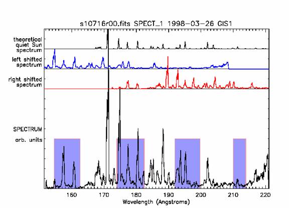
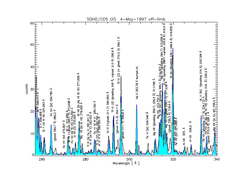
Figure 3a shows a portion of the GIS 1 spectrum, as an example. It is not only impossible to define a line profile, but even hard to recognise the presence of weak lines. Fixed patterning should not alter the total counts recorded in an emission line; it merely displaces some of them.
For some lines, the cluster of photon events will tend to spread across to the neighbouring arms of the spiral. This happens when the width of the spiral is broadened by electronic noise. This effect tends to occur only in those regions where the spiral arms are close together, and can lead to spreading to one of the adjacent arms (or both).
|
|
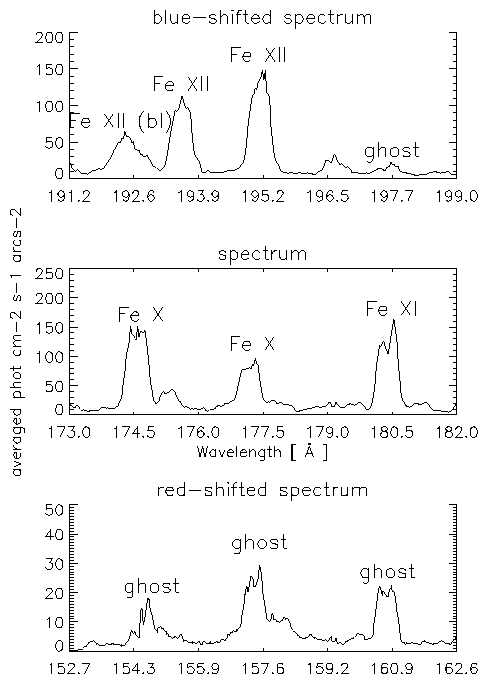
Now, once a set of LUTs is applied to the data on-board, i.e. a particular spiral pattern is assumed appropriate for the data, the original information is lost. In terms of counts versus wavelength, this means that a portion of the counts belonging to a line can be shifted into different parts of the telemetered spectrum, giving rise to spurious spectral lines if they fall in a spectral region void of lines, or providing extra intensity to already existing spectral lines. Henceforth we will refer to a spectral line whose intensity is enhanced in this way as ghosted (or contaminated) line, while the lines whose counts have been partially shifted toward other regions of the spectrum will be referred to as ghosting (or parent) lines. The counts shifted by this effect will be called ghosts, while the process will be called simply ghosting.
Since the spreading can only occur toward one or the other side of a spiral arm, each line can generate no more than two ghosts. When the spreading occurs toward the outer arm, a ghost is created at a lower wavelength, in the so-called red-shifted spectrum. Conversely, when part of the counts of a line are read into the inner arm, a ghost is created at a higher wavelength (in the so-called blue-shifted spectrum). Note that the definitions of red-shifted and blue-shifted GIS spectra do not have any relation to physical blue- or red-shifts, nor these spectra are simply `shifted' (in fact, they are compressed or expanded in the wavelength scale).
For each application of a given set of LUTs, ghosts will appear in the same positions. Once the applied LUTs are known, it is therefore possible to deduce which regions of the spectrum are unlikely to be affected by them, and to predict where ghosts might appear. It is therefore theoretically possible to deghost (or reconstruct) the spectra, i.e. add to each line the intensity lost by the creation of a ghost.
Unfortunately, the situation is quite complex, for many reasons.
|
|
|
An important aspect of the planning of CDS observations comes in the designing of the `studies' to be run by the instrument. Each CDS study is a sequence of commands to be sent to the spacecraft, containing
pointings
exposure times
movements of the mirror and/or the chosen slit
various telemetry instructions (for example the specifications of the extraction windows for the NIS).
See. e.g.
mk_raster
mk_study
CDS 'raw' data from each raster are stored in FITS files as binary tables. Routines expect to find the data in the $CDS_FITS_DATA directory.
The data can be loaded into IDL memory into the so-called quicklook data structure (QLDS), a 'special' CDS-specific entity:
a=readcdsfits(file)
Normal IDL commands MUST NOT be used. for example, to copy:
qlds = copy_qlds(a)

; b=a WOULD NOT WORK !!!
;----------------------
To DELETE the QLDS from memory:
 delete_qlds,qlds

; delvarx, QLDS WOULD NOT WORK !!!
;--------------------------------
Once the data have been loaded, the QuickLook package can be used to inspect (and analyse) them:
dsp_menu, qlds
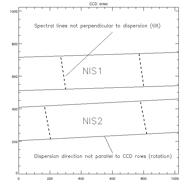
The VDS detector is mainly composed of a microchannel plate and a 1024x1024 pixels charge coupled device (CCD), composed of four square sections. The CCD was orientated with its columns parallel to the slit alignment. Therefore, any pixel Y position should represent a single Solar Y point, while the grating dispersion is along the pixel X coordinates. In reality, the CDS alignment is more complex, as shown in Figure 3.6.1 and described below.
A pixel in the detector Y direction corresponds to 1.68óó. The extent in Y of the long slits (240óó) is therefore 143 pixels on the detector.
A pixel in the dispersion (X) direction corresponds to about 0.07 Å for NIS 1 and 0.11 Å for NIS 2.
lw = gt_wlimits(qlds, /short)
Window        Label         Band    Xmin   Xmax    Wmin      Wmax

  0       O_4_554_51        NIS2    344    368    553.13    555.93
  1       HE_1_584_33       NIS2    599    623    582.94    585.75
  2       O_3_599_60        NIS2    729    753    598.17    600.99
  3       MG_9_368_07       NIS1    850    874    367.22    368.91
  4       MG_10_624_94      NIS2    945    969    623.52    626.34
  5       O_5_629_73        NIS2    986   1010    628.34    631.16
The Xmin Xmax numbers give the detector start and stop pixels for each data window. The wavelengths are calculated using an average pixel-wavelength conversion applicable to the date of observation. The table above also shows that the data windows are 25 pixels wide.
To put the data of the first window into an array:
data = gt_windata(qlds,0)

help,data
DATA            FLOAT     = Array[25, 10, 73]
The wavelength dimension has 25 pixels, 10 exposures were taken by stepping in SolarX, and only 73 pixels along the slit (SolarY) were telemetred.
In general, the variable data will then be a data array with from 2 to 4 dimensions. The dimensions are always in the order (Wavelength , SolarX, SolarY, Time). The fourth dimension (Time) is only added where the observation sits at the same SolarX location and takes repeated exposures. In that case the SolarX dimension is retained, but only has one element.
If you are interested in comparing actual timings for the events as seen by different instruments, you need to get the starting time for each of the exposures (i.e. slit positions):
time_start=gt_start(QLDS,/exposure,/truncate)
Unfortunately, the NIS spectra contain a large scattered light ( `background' ) component when observed on the solar disc. The main contributors are probably the Lyman-alpha and the Lyman continuum.
The NIS 1 spectral region, where CDS has many potential diagnostic lines, is the most affected. This scattered light produces a spatially and wavelength-dependent background component in the spectra, and is most intense in the network spectra.
Typically, in the NIS 1 channel, the scattered light component is a factor of 2 higher in the network areas than in the cell centre areas. The background level can be of the order of the peak intensity of most of the NIS 1 lines in coronal hole regions, and also in the quiet sun.
The background determination provides the major uncertainty in line intensity measurements.
It is basically only important in off-limb observations. Some pre-flight information is available in Harrison et al (1995), Solar Physics, 162, 233. which gives results for measures at a wavelength of 68 Å.
See also David et al (1997), Fifth SOHO Workshop, SP-404, Page 313.
Routines to calculate the amount of scattered light and an explanation of how to apply them are available at:
ftp://www.medoc-ias.u-psud.fr/pub1/softs/david/
This is accomplished by the CDS routine VDS_DEBIAS:
vds_debias, qlds
Unlike the GIS detectors, the VDS is not a photon counting device, so describing the data as ``counts'' is inappropriate.
Normally NIS studies are designed to include four VDS background windows in the corners of the CCD. Average CCD readout biases can then be removed by VDS_DEBIAS from each of the four CCD sections. The error associated with this step is small (1 in ADC units, ~ 0.5 photon-events/pixel) when compared to the scattered light. Raw data from the VDS detector are in `ADC' (Analog to Digital Conversion) units. After applying VDS_DEBIAS, the units of the data are `DEBIASED-ADC'.
See CDS software Note 46: Missing Pixels and Cosmic Rays for details.
An effect that strongly constrains the observations is the presence of cosmic ray hits. Exposure times cannot be too long, otherwise cosmic rays literally wipe out the use of large fractions of the spectra. Various software routines are available to automatically `flag' cosmic ray hits with `missing' values, but an interactive check is highly recommended, although this takes a very long time if the number of exposures and extraction windows is large.
An useful GUI is XCDS_COSMIC which allows to use e.g. CDS_CLEAN_EXP (OK for pre-recovery not Y-binned data) or CDS_CLEAN_SPIKE
Important NOTE: you will need to have defined $CDS_EXTERNAL to point to a compiled version of external.f if you are going to use CDS_CLEAN_EXP.
xcds_cosmic,qlds
Figure 3.6.1 shows some cosmic ray hits flagged as missing with this software. Often, the number of cosmic ray hits is such that a line profile in one exposure is lost and no line intensity can be deduced. Therefore, it is highly recommended to raster small regions on the sun a few times, clean the single spectra from the cosmic rays, and then average the spectra. In this way, the effect of the cosmic rays is removed (unless cosmic rays hit the same emission line at the same spatial position along the slit). Another way of reducing the effect of the cosmic rays is to spatially average the line profiles.
Important note: the standard CDS_CLEAN_IMAGE does not work properly for Y-binned data, nor when strong brightenings (or small flares) are present in the data.
Data must be visually inspected.
Details are given in CDS software note 51.
The flat field of the detector presents variations of only a few percent. However, before the spectra are divided by the appropriate parts of the flat field, the burn-in correction is added to the flat field. The VDS detector sensitivity decreases with time in the most strongly illuminated areas (i.e. in the centres of the brightest lines), because of local gain depression, a well-known effect in NIS (called burn-in). This has been monitored since launch using wide slit observations.
In fact, the burn-in of all the isolated lines can be accurately estimated from the images obtained when the instrument is operated in spectroheliogram mode with the 90x240 arc sec slit. Such images show a marked depression of the line intensity at the core of the line.
|
|
The line profiles are reconstructed, adding to the flat field some gaussian `absorption' profiles with a predicted width, position, and normalized peak intensity. Table 3.5 shows some of the lines that need such a correction. Note how the correction changes with time, and how considerable it is. For example, the He I 584 Å line, the brightest in these detectors, had already in September 1997 a burn-in of 40%. This correction is accurate (to a few percent) only for the bright and un-blended lines.
|
| |||
| Line | Detector | 1st Sept 1997 | 1st Sept 1996 |
|
| |||
| Fe XVI (bl) 335.407 Å | NIS 1 | 0.141 | 0.095 |
| Fe XI 341.117 Å | NIS 1 | 0.005 | - |
| Si X 347.390 Å | NIS 1 | 0.080 | - |
| Si X 356.023 Å | NIS 1 | 0.081 | 0.006 |
| Fe XVI 360.763 Å | NIS 1 | 0.165 | 0.093 |
| Fe XII 364.456 Å | NIS 1 | 0.096 | 0.051 |
| Mg IX 368.086 Å | NIS 1 | 0.226 | 0.146 |
| O III 525.863 Å | NIS 1 | 0.104 | 0.050 |
| He I 537.108 Å | NIS 2 | 0.161 | 0.112 |
| O IV 554.499 Å | NIS 2 | 0.236 | 0.146 |
| He I 584.370 Å | NIS 2 | 0.419 | 0.321 |
| O III 599.620 Å | NIS 2 | 0.124 | 0.082 |
| Mg X (bl O IV) 609.818 Å | NIS 2 | 0.268 | 0.158 |
| Mg X 624.990 Å | NIS 2 | 0.189 | 0.099 |
| O V 629.819 Å | NIS 2 | 0.369 | 0.274 |
The NIS1 readout electronics create a low-level fixed-pattern effect in the spectrum. Every fourth pixel appears to have a lower count than expected. The effect is corrected by the routine VDS_CALIB.
VDS_CALIB, after dividing the spectra by the flat field, corrects the exposure time and divides it into the data to give the ADC count rate. The correction to the exposure time is due to the electronic shuttering, which makes each exposure slightly longer (0.1165 seconds for the normal VDS operating voltage).
VDS_CALIB also applies a correction for non-linear effects at high count rates (ADC counts per photon, a function of the voltage). These corrections are large for high count rates.
Then, the VDS throughput is divided into the data to convert from DEBIASED-ADC count-rate to photon-events/pixel/s. The term ``photon-events'' refers to those EUV photons which actually interact with the detector.
For subsequent data analysis, it can be useful to have the spectra in photon-events/pixel and so the output from VDS_CALIB should be multiplied by the `corrected' exposure time.
Exposure durations:
The exposure durations are given in the parameter QLDS.HEADER.EXPTIME in the quick-look data structure. Strictly speaking, one should really multiply by the corrected exposure time, which is slightly longer than that given in the header. However, this correction is very small (0.1165 seconds for the normal VDS operating voltage), and can safely be ignored in most cases.
vds_calib, qlds, exptime_corr=exptime_corr,THROUGHPUT=THROUGHPUT

; QLDS now has units  PHOT-EVENTS/PIXEL/SECONDS
;if you want COUNTS/PIXEL/S  multiply for THROUGHPUT

;if you want PHOT-EVENTS/PIXEL multiply by exptime_corr
Unfortunately, it is not possible to make in-flight adjustments to CDS to correct for, e.g. distortion during launch. This has resulted in a series of effects, that can only be partially corrected for during the data analysis.
First, it seems that the NIS instrument is not in focus. In fact, the line widths created by the 2óó and 4óó slits appear to be about the same, and much larger (by factors ~ 2) than in pre-flight measurements. No correction is possible.
Another optical factor to take into account in the data analysis is the fact that the centres of the various slits are not co-aligned, which has the consequence that images taken will not be aligned in the Y-direction. However, images taken with different slits by the author show that the 4óó× 4óó and the 4óó× 240óó slits are co-aligned, in accordance with results based on other work (D. Pike, priv. comm.), which have shown for the other slits misalignments of up to 4óó.
Then, the spectra are slanted, in the sense that the dispersion direction is rotated relative to the rows of the VDS CCD, with different angles for NIS 1 and NIS 2, as shown in Figure 3.6.1. This is the main effect, and is caused by a slight misalignment between the grating and the detector.
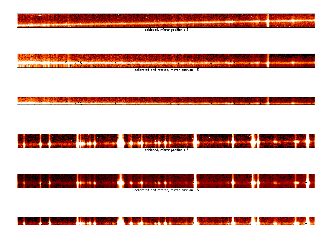
| #1 The NIS spectra, showing the effects of the slant of the spectra and the cosmic rays. First three spectra, from top to bottom: a NIS 1 de-biased spectrum; the same spectrum with the cosmic rays flagged as missing data, calibrated using VDS_CALIB (and NIS_CALIB), and rotated (using VDS_ROTATE); the previous spectrum, but with the unusable spatial areas (top and bottom rows) removed. The bottom three figures show the NIS 2 spectra. The particular exposure shown here was taken during a brightening in a spatially-localized region of the network. The bright stripe across the spectra is caused by enhanced emission in all the emission lines, plus by scattered light, and clearly shows the slant of the spectra, that is more pronounced in NIS 1. Note that a large portion of the spectra (along the slit) is lost after the correction for the slant is applied. |
It implies that a row of CCD pixels covers different SolarY values at different wavelengths.
On top of this, the spectral lines are tilted relative to the dispersion direction (i.e. the angle they for with the dispersion direction is not 90 degrees, and varies). It is caused by a small misalignment between the grating and the slits. It implies that the position of a spectral line (measured in CCD x-pixels) will vary along the slit (SolarY direction) and would give a false velocity variation in the N-S direction.
|
|
The slant of the spectra complicates the planning of a CDS `study' and data analysis.
A correction for the slant and tilt of the lines can be done in two ways, one during the data planning and one in the analysis (by the routine VDS_ROTATE).
During the planning of a CDS `study', the CDS routine MK_RASTER makes the following adjustment. If a study is designed with specific data extraction windows then the windows are positioned on the detector at different row positions to allow for the slant. Hence pixels along the slit of different data windows correspond (within one pixel) to the same solar location and the correction for the slant of the lines is not necessary, although the approximation is about one pixel in Y. Using this method, data extracted at any of the wavelength windows are co-spatial on the Sun to within one pixel in Y. [The usual extraction window height is 143 pixels, corresponding to 240óó.]
For studies that use the full default extraction window the correction for slant has to be applied during data analysis, and it is important in the planning phase to extend the Y-size so that a sufficiently large area of the detector is extracted, to cover the full rotated spectrum. In the data analysis, VDS_ROTATE is used to rotate the entire NIS 1 and NIS 2 spectra to correct for the slant and tilt. In this category there are two further types of CDS `studies', one that extracts the full spatial positions along the slit (as done in the spectral atlases) and one with a shortened extraction along the slit (case shown in Figure 3.6.1).
In the case of spectral atlases, two windows of 1024x160 pixels are extracted. VDS_ROTATE pivots around the centre of the data. There is a difference in the height of the unrotated data for NIS1 and NIS2, where the first is 160 pixels in height, and the second is only 153 pixels. Therefore, NIS1 data pivots around vertical pixel 79.5, while NIS2 data pivots around pixel 76. Thus, there is a 3.5 pixel difference in the positions due to that effect. VDS_ROTATE then cuts the two spectra to 143 pixels, although two arrays of 1024x160 pixels are given in output. However, when the /BOTTOM keyword is used, then the bottom of the slit is aligned with the bottom of the array, and the data should be directly comparable.
In the other case, with shortened extraction along the slit, there is no difference in the height of the unrotated data for NIS1 and NIS2, and the spectra are rotated around the centre of the data.
In any case, the slant of the two channels is such that about 30óó along the slit direction are lost, if one is interested in having all the NIS spectral information at the same spatial position. Figure 3.6.1 shows the rotated NIS 1 and NIS 2 spectra.
The tilt of the lines can be partially corrected for by applying the routine VDS_ROTATE (or NIS_ROTATE) to the spectra, or by adjusting the wavelength calibration.
Note:
NIS_ROTATE, QLDS
Finally, note that the spectral line tilt may have changed post-recovery.
Both NIS1 and NIS2 use the same entrance slit to the spectrograph. However, there appears to be a N/S offset, sometimes amounting to several arcseconds, between the solar features that NIS1 sees and those that NIS2 sees. The effect seems to depend on the Solar Y position.
|
|
The effect is more pronounced in post-recovery data and could amount to ~ 7 pixel vertical shift between NIS-1 and NIS-2 images.
Use the routine gt_nis_alignment which returns the best estimate of the offset.
There is also an offset between the imaging of NIS and GIS. GIS images appear approximately 13" south of their NIS equivalents. Specific (X,Y) pointings for GIS should therefore be 13" south of the values determined by the software
Although nominally CDS has a fixed wavelength range, small changes in the zero point of the pixel-wavelength relation can occur, primarily from on board temperature changes caused by varying illumination of the structure by the Sun. The wavelength array returned by the gt_xxxx functions or the pix2wave function is only an average determined from sample spectra. For accurate wavelength analyses, the zero point should be determined from each spectrum individually.
The calibration appropriate to a particular dataset is loaded when the data file is read. If you want to know what the currently loaded coefficients are, use the routine
IDL> qwavecal
The slant of the two channels, and the tilt of the lines complicates the wavelength determination.
The NIS wavelength calibration also has some peculiar aspects. The wavelength calibration requires a `scan mirror correction', which appears to be different for different observations. Then, the NIS wavelength calibration has been found to be a function of the CDS optical bench temperature (D. Pike, priv. comm.) and its history, which continuously changes depending on the solar illumination. It has been observed to cause shifts of up to a pixel (0.1 Å), which for a strong line such as O V 629 Å corresponds to a velocity of 56 km/s.
In conclusion, NIS does not have an accurate `standard' wavelength calibration, and therefore, in the absence of any reference wavelength scale, most absolute wavelength measurements are subject to various uncertainties. Also, the NIS shows a series of geometrical effects that are not well understood and are difficult to explain, and can only be partially corrected for.
In practice, a simple way to extract an array of wavelengths `w' for each NIS window is:
; get the array w  of wavelengths for the first (0) window,
; corresponding to the first spatial position (xix=0,yix=0)

dummy=gt_spectrum (qlds,WINDOW=0,xix=0,yix=0,lambda= w)

;once obtained, it might be useful to plot an averaged spectrum:

; average over the Solar X,Y:

sp=average(average(data, 2, missing=-100),2, missing=-100)

window,0 & plot, w,sp,psym=10
For details, see:
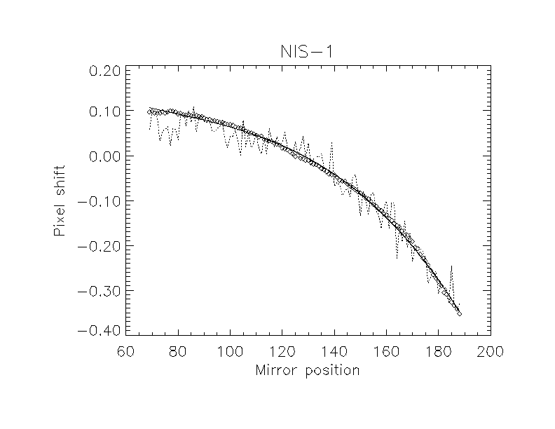
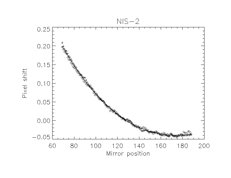
http://orpheus.nascom.nasa.gov/~thompson/slit_inten/mirror_position.html
|
|
|
|
The pixel shifts derived by Bill Thompson from the above data are:
DPIX = POLY(MIR_POS-128, [0,-0.0030423011,-3.3262600e-5,-2.0959131e-7]) ;NIS-1
DPIX = POLY(MIR_POS-128, [0,-0.0018515786, 2.3390659e-5,-4.0578093e-8]) ;NIS-2
An early demonstration of the effect of CDS optical bench temperature on the NIS wavelength zeropoint. The temperature varies as a result of different illumination conditions caused by changing the CDS pointing. These results are taken from analysis of the OV 630A line in the daily synoptic scans. The dots show the recorded optical bench temperature and the open circles the pixel centroid of the OV line. Prior to 12-Jun-96 a reasonable correlation can be seen. On that date the stabilisation temperature was raised to 23 Deg. C ie it was held above the peak of its natural level. Since then the temperature and the wavelength zeropoint have been very stable, although some analysis hints that a small temperature dependence still remains. See SYNOP_STAB_DEMO. The sharp drop in temperature around 28-Jun was caused by closure of the CDS doors for station keeping manouvers.
|
|
Even after all the possible tilt and wavelength corrections, the line profiles are not strictly gaussian, and residuals to gaussian fits show peculiar spatial patterns still not explained.
It has to be noted that the resolution of the instrument (FWHM of the Point Spread Function or PSF) is at least 5-6óó. Therefore, the pixel resolution (1.68óó) along the slit is much less than the spatial resolution, and the spectra can be binned without losing any spatial information.
Following suggestion from the author, many CDS studies have been designed and used to perform Y-binning on-board, to reduce telemetry time.
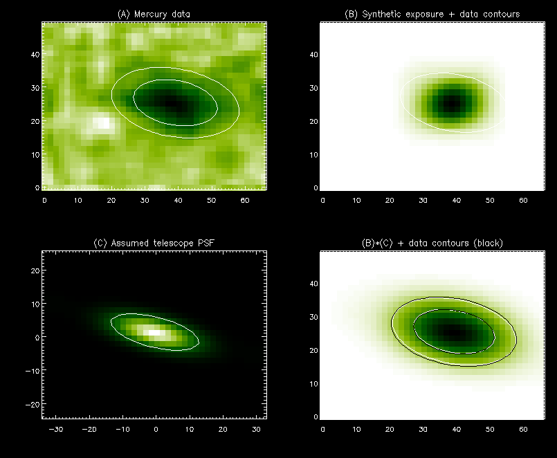
S. V. H. Haugan discusses in Anomalous Line Shifts from Local Intensity Gradients on the SOHO/CDS NIS Detector (Solar Physics 185, 275, 1999) the NIS PSF. He suggests that the NIS spectrograph PSF must be slightly elliptical and rotated.
Pauluhn, A. et al., 1999, Applied Optics 38, 7035, also discuss the issue, deriving the pre-loss Point Spread Function (PSF) for CDS/NIS from a comparison with Sumer data. They suggest a slightly elliptical form with FWHM(x) = 6" and FWHM(y) = 8" (when the 4"x240" slit is used).
The post-recovery PSF has apparently degraded. See details in the CDS user guide.
|
|
From launch to the loss in June 1998, the CDS/NIS line profiles were very approximately Gaussians.
The CDS preflight calibration came up with the following numbers for the line half-widths in pixels:
        Slit    NIS1            NIS2
        4       3.4 +/- 0.3     3.2 +/- 0.2
        5       3.7 +/- 0.4     3.7 +/- 0.2
the line width in both bands is about 4.3 pixels FWHM with slit 4 and only slightly wider with slit 5, about 4.6 pixels.
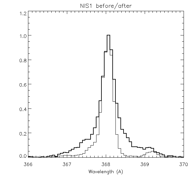
After recovery the NIS line profiles have changed. The bakeout that CDS suffered during the SOHO loss changed the line profiles produced by the NIS spectrometer. The NIS1 profiles exhibit broader wings and the NIS2 profiles show a broadened and asymmetrical long wavelength wing.
See Software note #53 for details on the effect and on the broadened gaussian asymmetric profiles.
|
 |
The best multiple-line-fitting IDL software is the CFIT package, created by Stein Vidar Haugan, and described in Software note #47.
Line profiles can have any general shape, and the `background' is normally fitted with a polynomial. Any number of parameters can be fitted; any number of lines can be fitted over a wavelength region.
The parameter's values can be allowed to vary within some fixed ranges, or can be kept constant. In many cases lines are closely spaced, and a proper de-blending can only be done if ranges for the positions and widths are given.
Each fitted line's parameters can be checked and modified interactively. The fit is performed with a non-linear weighted least squares fit, optimizing an initial user-supplied set of parameters in order to find the best agreement between the chosen model function and the observed data.
The data are given `weights' 1/s2, where the s is the noise associated with the data, s = ų(N) where N is the total number of photon-events/pixel.
The fitting is done passing a series of initial parameters that define each line to be fitted.
Only `real' lines that have a width at least equal to the instrument resolution should be fitted. This can be done by fixing the minimum line width equal to the instrument resolution.
An entire book could be written on this issue. For details, see the first (and still only) comprehensive in-flight calibration of all 9 CDS channels:
Del Zanna, G., et al., 2001, A&A 379, 708-734. Solar EUV spectroscopic observations with SOHO/CDS. I. An in-flight calibration study
Also, see the book:
The Radiometric Calibration of SOHO, ISSI Scientific Report, 2002, Pauluhn,A., Huber M.C.E., von Steiger,R. eds.
And my WWW pages:
http://www.damtp.cam.ac.uk/user/astro/gd232/cds/
The CDS routine NIS_CALIB performs the conversion from photon-events/pixel/s to the calibrated default units `photons/cm2/sec/arcsec2'.
The conversion factor from arcsec2 to steradians is simply (p/(180 ×602))2 @ 2.35 ×10⁻¹¹, while the conversion from photons to ergs is hc/l @ 1.986×10⁻⁸/l, where l is in Ångstroms. The conversion to per Ångstrom is accomplished simply by dividing the data by the pixel width in Ångstroms.
There are several factors which determine this final conversion of the data from photon-events to absolute units.
The absolute sensitivity ef(l) [counts/photons] as a function of wavelength.
The absolute sensitivity of the NI spectrographs is a combination of:
the reflectivity of the primary mirror, the secondary mirror and the scan mirror;
the efficiencies of the gratings;
and the quantum sensitivity of the VDS detector.
The wavelength dependence of absolute sensitivity is therefore a combination of the wavelength dependence of all these various factors.
The following table shows the progress of the various calibrations implemented within the software:
    Version     Date        Notes

1    16-Sep-1996    Original calibration, based on pre-flight absolute
                    measurements and in-flight line ratios.

2    23-Dec-1998    Modified calibration, based on EGS sounding rocket
                    measurements and reanalysis of the pre-flight data.

3    28-Feb-2000    Modified NIS-1 calibration, based on SERTS and EGS
                    sounding rocket measurements.  NIS-2 curve unchanged.

4    21-May-2002    Modified NIS-2 calibration, based on reanalysis of EGS
                    sounding rocket measurements.  Incorporated
                    second-order NIS-2 curve.  Modified GIS calibration
                    curves.
It is important to note that any raw data run through the current software will use the LATEST calibration values irrespective of the observation date, but instrumental effects (eg MCP burn in) will depend on both the actual observation date, and the time when the latest corrections have been put into the database (hence on when you analyse the data).
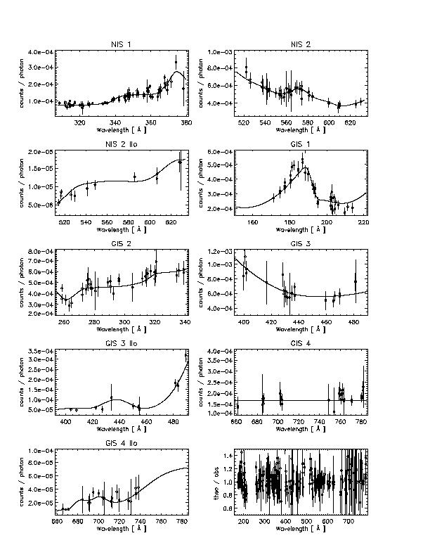
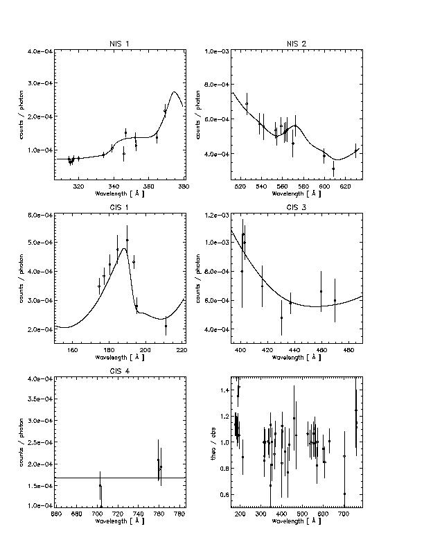
Figures from Del Zanna et al. (2001) and my WWW pages.
|
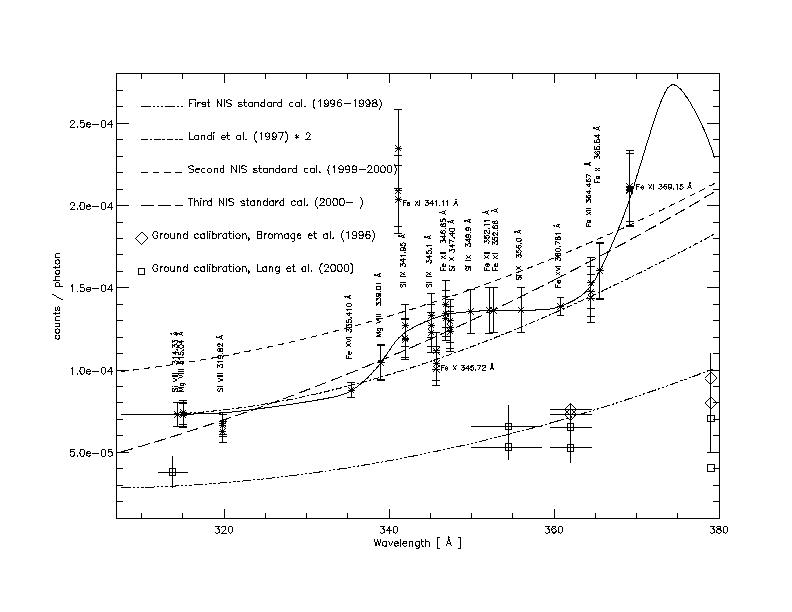
Excellent agreement is found between the calibration presented here and the other two independent in-flight studies based on rocket flights in 1997. In particular, the values of the calibration presented here almost coincide at 368 Å with the only reliable absolute NIS 1 measurement of Brekke et al. (2000). Significant discrepancies with the ground measurements are found.
|
Very good agreement with the calibration proposed here is found, in particular at 320 Å and in the region 339-353 Å. The main disagreement concerns the lines that have been labelled, AL X 332.8 Å, Fe XIV 334.2 Å, and Fe XVI 335.4 Å. The CDS and SERTS-97 observed a very bright active region, and these lines were the most prominent ones in the SERTS-97 spectrum (indeed the measurement error is very small). The observations were made at a location with steep spatial gradients in the hottest lines, and any small spatial misalignment between the two instruments would mostly affect these three lines, that are the higher temperature lines in the SERTS-97 spectrum (R.J. Thomas, 2001, priv. comm. - further work is in progress).
|
The only direct in-flight absolute calibration study is that of Brekke et al. (2000). In considering a detailed comparison with the diagnostic study presented here, it should be noted that the coarse resolution ( @ 5 Å) of the rocket flight spectrum limited the evaluation of the instrumental background, increasing the uncertainty. The spectra have been binned into six wavelength regions, and the background estimation was very difficult.
The downturn at wavelengths below 530 Å is regarded as uncertain by Brekke et al. (2000), because of low signal. The region 590-610 Å proved difficult to fit and was not used by Brekke et al. (2000). Considering the above, these results and Brekke et al. (2000) ones are very much consistent.
Note that neither the ground calibration measurements nor the theoretical predictions of the sensitivities are in accordance with both the direct in-flight results of Brekke et al. (2000) and those presented here. In particular, there is no agreement with the He I lines.
Finally, it is interesting to note that the calibration proposed here would partly explain the discrepancies that were found when the SUMER detector A and the NIS calibrations were compared in-flight at 584, 610, 625 Å (see Pauluhn et al., 1999).
|
|
|
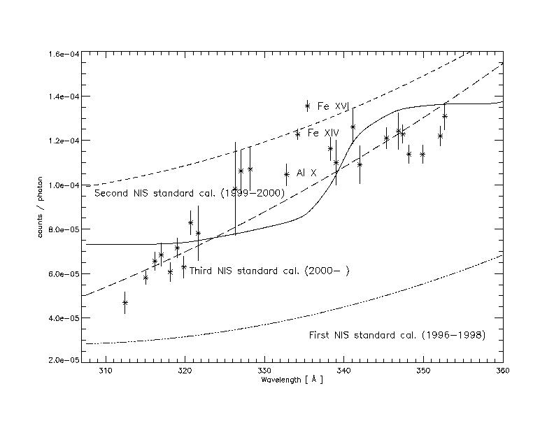
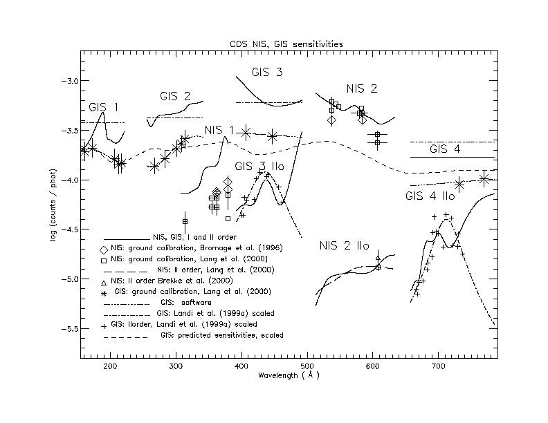
The main features of the calibration presented here, compared to the previous studies are:
Some differences with the predicted second order sensitivities at the other wavelengths are found.
Note, however, that the absolute values of the predicted sensitivities are about a factor of 10 higher than the values presented here.
|
No significant changes in the calibration appear to be present from a single dataset (Del Zanna et al. 2001). However, there are many indications that the sensitivities have changed, in particular the NIS 1 one. See the book on the SOHO radiometric calibration.
The telescope aperture At(k) [cm2].
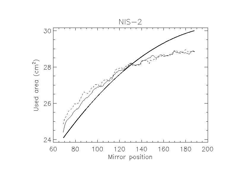
At(k) is a function of the scan mirror position (k), because as the scan mirror moves, the two NIS gratings are `seeing' different parts of the NIS telescope aperture.
The variations, around a median value of 27-28 cm2 (for NIS 1-2) are considerable ( ~ 20%) over the full extent of the scan mirror positions (4ó). The CDS routine GET_EFF_AREA provides the pre-flight values of At(k), and these have been confirmed by in-flight measurements (W. Thompson, priv. comm.).
|
|
The geometric area available at the slit, that depends on which slit is used.
The exposure time.
For details, see:
http://orpheus.nascom.nasa.gov/~thompson/slit_inten/slit_intensity.html
There is evidence of an intensity gradient along the slit in VDS data. Furthermore, the variation appears wavelength dependent.
It's unclear what is causing this effect. It is probably generated within the instrument optics, either within the telescope or in the two NIS gratings.
Bill Thompson analysed NISAT_S, NIMCP, and SYNOP_F data and came up with the following conclusions. The behavior along the slit falls into two classes. One class behaves like Mg IX 368, where the intensity increases as one goes from the bottom of the slit to the top. The other class behaves like O V 630 A, where the intensity descreases as one goes upward from the bottom of the slit, and then levels off. Other lines, such as He I 584 A, can be modelled as a linear combination of these two behaviors.
|
 |
 |
There are many ways of dealing with this issue. I recommend to analyse the 'raw' data, and apply the radiometric Calibration only at the end.
One possible way to do this is to create a 'dummy' QLDS, fill the data with unity values, and then apply the Radiometric Calibration. In this way, you will have arrays with the correction factors, that you can inspect and eventually modify.
qlds_calib=copy_qlds(qlds)

NWIN = N_ELEMENTS(QLDS_CALIB.DETDESC)

; fill the data with unity values:
;----------------------------------

FOR IWIN = 0,NWIN-1 DO BEGIN  &$
ARRAY = DETDATA(QLDS_CALIB, IWIN+1)  &$
ARRAY[*]=1.  &$
ST_WINDATA,QLDS_CALIB,IWIN,ARRAY,/NO_COPY  &$
ENDFOR


; apply the calibration:
;-----------------------

nis_calib,qlds_calib, /ERGS, /STERAD

;     The default units for the returned data are
;        PHOTONS/CM^2/SEC/ARCSEC^2, but
; since we used the /ERGS, /STERAD keywords, the
; unints are  ERGS/CM^2/SEC/STERAD
;------------------------------------------------
The various noise sources associated with the NI spectrometers are described in detail in the CDS Software Note #49: Deriving Statistics from NIS data.
As well as Poisson noise associated with the photons which interact with the detector, there is another source of noise due to the fluctuation in the amount of amplification in the detector system, known as the pulse height distribution (PHD). This latter effect can be assumed to be comparable to the Poisson noise. Other sources of noise are only detector-dependent. The readout noise R has been found to vary from 0.62 to 0.83 photon-events/pixel, and therefore has an effect only at low light levels. A value of 0.7 is assumed in this work.
Another major effect is that the detector resolution makes each photon affect more than one pixel on the CCD. The line profiles therefore appear smoother than would be expected from the photon statistics, and it is more appropriate to consider the statistics of the whole group of pixels where each line is spread.
This makes error estimates based on curve fitting appear smaller than the true values, in many cases.
If N is the total number of photon-events in a line, the Poisson noise is ųN, and assuming that the PHD component is comparable, and adds in quadrature, the total photon noise is sN = ų{2*N + R2*npix}, where npix is the number of pixels being summed over and R is the readout noise per pixel. In reality, the main source of error in determining intensities in NIS spectra is the scattered light in the detector, and what we want to measure is the intensity of each background-subtracted line I=N-B , where B is the total background intensity over the line. The noise associated with the background is again sB=ų{2*B + R2*npix} and the error on the intensity I is therefore
| (1) |
In the case of navg spectra averaged, we have to divide sI by ų{navg}.
Another way to determine the error on the intensity is directly from the errors on the parameters of the fit. If the line profile is gaussian, the total intensity in the line is derived from the peak amplitude I0 and the line full-width-half-maximum FWHM (in pixels):
| (2) |
Since the peak amplitude I0 and the FWHM are not statistically independent, in the sense that too high FWHM favors too low I0 and vice versa, the error on the intensity sI can be calculated from:
| (3) |
For unblended lines the errors calculated in this way are similar to those calculated from the total line intensities.
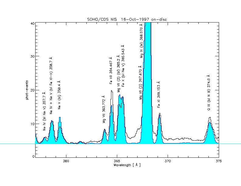
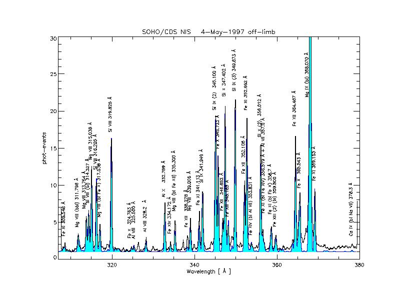
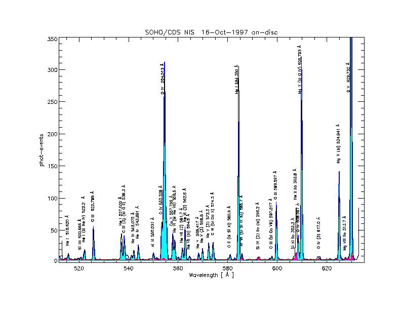
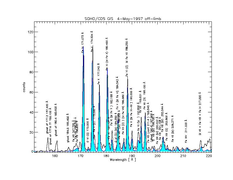
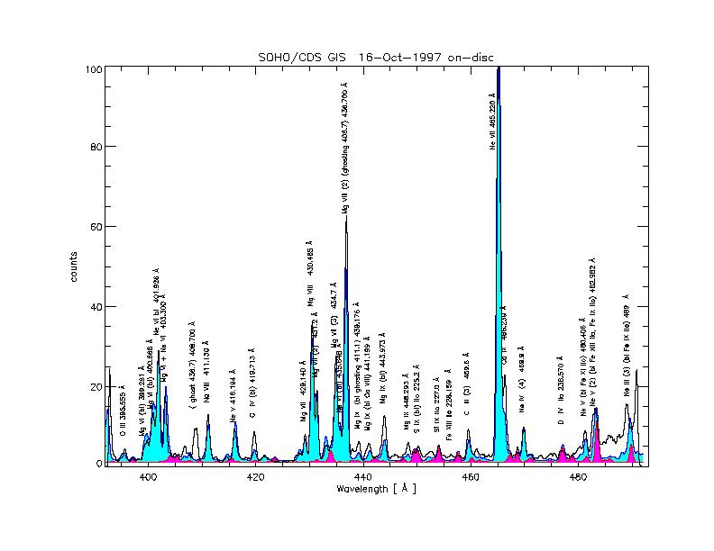
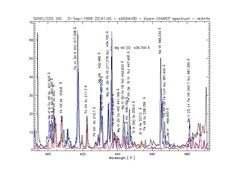
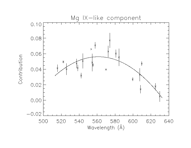
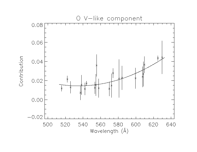
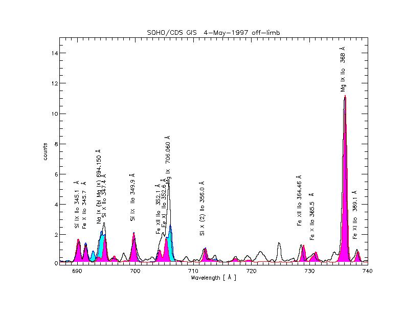
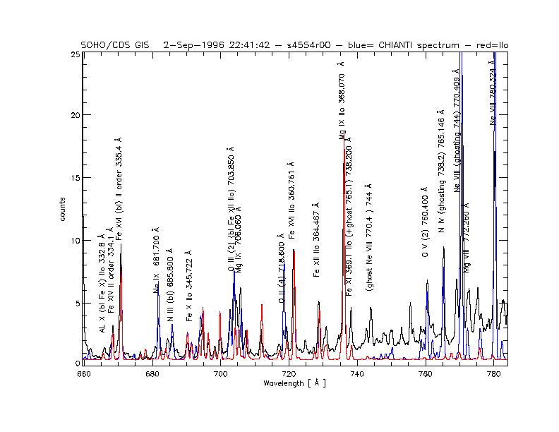
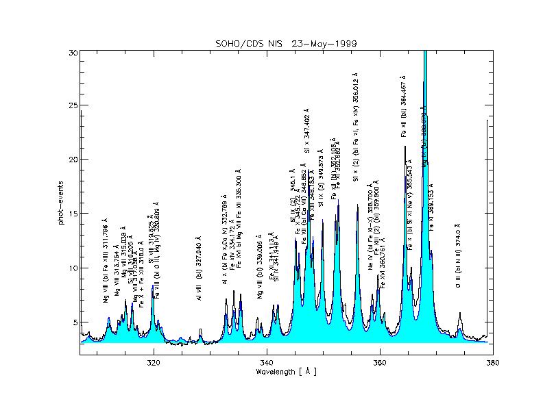
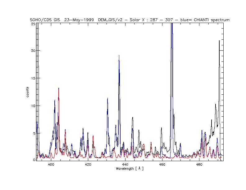
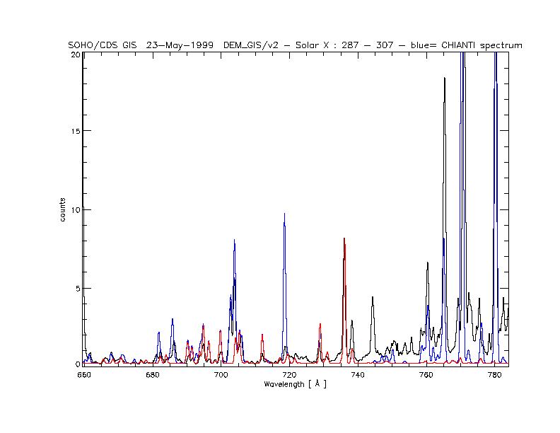
Now, a list of observed spectra (black), with superimposed CHIANTI synthetic spectra (blue +shaded areas), with second order contributions (red +shaded areas).
|
|
|
|
|
|
 |
|
 |
|
 |
|
 |
 |
 |
 |
 |
 |
The best way is to use Dominic Zarro's map structures. For details, see
http://orpheus.nascom.nasa.gov/~zarro/idl/maps.html
and the EXERCISE section.
There is no complete CDS line list. The only published line list is a quiet-Sun NIS line list (which does not include most second order lines) from Brooks et al. (1999).
The only almost-comprehensive GIS and NIS line lists are to be found in my PhD thesis. However, they are not complete, and some line identifications of the weaker lines need to be revised.
You can create your own line lists by using the CHIANTI user-friendly widget:
ch_ss ; , font=font
Detailed information on possible ways of handling GIS data can be found in the following CDS Software Notes:
54: CDS-GIS Instrument Guide (PostScript 3 Mb)
55: GIS Software User Manual (PostScript 465 Kb)
56: GIS Calibration Details (PostScript 1 Mb)
A different approach is suggested and described in detail in my PhD thesis and in various papers I wrote (see e.g. Del Zanna et al. 2001 and references therein).
For details, see e.g.: Mason and Monsignori Fossi 1994; Del Zanna et al. 2002; Del Zanna 1999.
Also the CHIANTI user guides that I wrote, which can be found in the WWW pages, e.g.:
RAL, UK: http://www.chianti.rl.ac.uk/
In the `standard model' for interpreting line intensities there are three fundamental assumptions that serve to simplify the problem considerably (these are within the CHIANTI models but also normally assumed):
The last one normally holds for the EUV lines that CDS observes (with the exception of the helium lines), while the major uncertainties reside in the unknown ionization state. This casts serious doubts on results that can be obtained with spectroscopic methods.
The intensity I(lij), of an optically thin spectral line (having filling factor=1) of wavelength lij (frequency nij = [ c/(h lij)]) is
| (4) |
where i, j are the lower and upper levels, Aji is the spontaneous transition probability, Nj is the number density of the upper level j of the emitting ion and h is the line of sight through the emitting plasma.
In low density plasmas the collisional excitation processes are generally faster than ionization and recombination timescales, therefore the collisional excitation is dominant over ionization and recombination in populating the excited states.
This allows the low-lying level populations to be treated separately from the ionization and recombination processes.
For allowed transitions we have Nj(X+m) Aji ~ Ne. The population of the level j can be expressed as:
| (5) |
See the CHIANTI routine PROTON_DENS for details on how to calculate N(H)/Ne.
For the basic CHIANTI model these processes are simply electron and proton excitation and de-excitation, and the generalised radiative decay:
| (6) |
Cije is given by:
| (7) |
| (8) |
where wi is the statistical weight of level i, k is
Boltzmann's constant, T the electron temperature, and qij
the electron excitation rate coefficient which is given by:
| (9) |
Within CHIANTI, we presently model the Photoexcitation and Stimulated Emission by assuming a a blackbody radiation field of temperature T*. The generalized photon rate coefficient in this case is:
| (10) |
where Aji is the radiative decay rate and W(R) is the radiation dilution factor which accounts for the weakening of the radiation field at distances R from the source center.
We also assume an uniform (no limb brightening/darkening) spherical source with radius R*:
| (11) |
where
| (12) |
The solution of Eq. is performed by the CHIANTI routine pop_solver.pro, which gives the fraction of ions in the state i.
The level populations for a given ion can be calculated and displayed with plot_populations.pro (but also see pop_plot.pro).
We rewrite the intensity as:
| (13) |
where the function
| (14) |
called the contribution function, contains all of the relevant atomic physics parameters and is strongly peaked in temperature.
gofnt.pro calculates these contribution functions.
Please note that in the literature there are various definitions of contribution functions. Aside from having values in in either photons or ergs, sometime the factor [ 1/(4p)] is not included. Sometimes a value of 0.83 for N(H)/Ne is assumed and included. Sometimes the element abundance factor is also included. Any of the above (or any other) variations also affect the definition of a line intensity in terms of the contribution function and the DEM. In the following we will refer to the functions C(T,lij,Ne) and G(T,lij,Ab(X),Ne) = Ab(X) C(T,lij,Ne) ( i.e. the contribution function that contains the abundance factor ).
If we define, assuming that is a single-value function of the temperature, the differential emission measure DEM (T) function as
| (15) |
the intensity can be rewritten, assuming that the abundance is constant along the line of sight:
| (16) |
The DEM gives an indication of the amount of plasma along the line of sight that is emitting the radiation observed and has a temperature between T and T+dT.
The CHIANTI routine chianti_dem.pro calculates the Differential Emission Measure DEM(T) using the CHIANTI database, from a given set of observed lines.
In the isothermal approximation, all plasma is assumed to be at a single temperature (To) and the intensity becomes:
| (17) |
where we have defined the column emission measure
| (18) |
Please note that in the literature many different definitions of Differential Emission Measures, Emission Measures and approximations can be found (see Del Zanna et al., 2002 for some clarifications).
The theoretical intensity ratios from individual ion species provide a measurement of electron density which is independent of any assumptions about the volume of the emitting region.
DENS_PLOTTER and TEMP_PLOTTER are high-level widgets for the analysis of density- and temperature-sensitive ratios of lines from the same ion. They allow inclusion of proton rates and photoexcitation. The calling sequence is simple:
IDL > dens_plotter,'o_5'
to study O V.
IDL > temp_plotter,'c_4'
to study C IV.
|
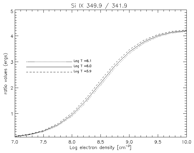
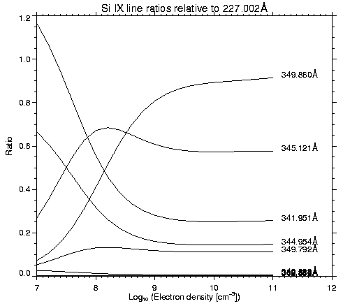
Figure 41 shows the density-sensitive Si IX ratio calculated at three temperatures (T=106 K is the temperature of maximum ionization fraction for Si IX), showing that these temperature variations do not appreciably affect the ratio.
The radiation that comes from the solar photosphere can excite transitions between levels in the ground configuration of ions in the corona, mainly affecting the level balance calculations for low densities (Ne Ż 108 cm-3).
The effect is stronger close to the photosphere, and tends to die out with height because of the decrease of the photospheric radiation field with distance. This decrease can be accounted for by estimating a geometric dilution factor that is a function of height above the photosphere. Si IX should be affected more than other ions.
|
| Ion | Ratio (Å) | Detector | log Tmax | log Ne | |
| Si IX (*) | 349.9 (3) / 341.949 | N 1 (G 4) | 6.02 | 7.5 - 9.5 | |
| Si IX | 345.100 / 341.949 | N 1 (G 4) | 6.02 | 7.5 - 9.5 | |
| Si IX | 349.9 (3) / 345.100 | N 1 (G 4) | 6.02 | 7.5 - 9.5 | |
| Si X | 356.0 (2) / 347.402 | N 1 (G 4) | 6.12 | 8.0 - 10.0 | |
| Fe XII | 338.278 (!) / 364.467 | N 1 (G 4) | 6.16 | 7.0 - 12.0 | |
| Fe XIII | 321.4 / 320.80 | N 1 | 6.21 | 8 - 10 | |
| Fe XIII | 318.12 / 320.80 | N 1 | 6.21 | 8 - 10 | |
| Fe XIII | 359.6 (2) (!) / 348.18 | N 1 (G 4) | 6.21 | 8 - 10 | |
| Fe XIII (*) | 320.8 (bl) / 348.18 | N 1 | 6.21 | 8 - 10 | |
| Fe XIII (*) | 203.8 (2) / 202.044 | G 1 | 6.21 | 8.5 - 10.5 | |
| Fe XIV | 353.83 (!) / 334.17 | N 1 (G 4) | 6.25 | 9.0 - 11.0 |
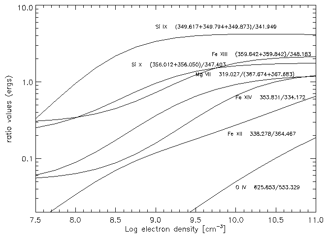
Table 2 presents a list of useful density-sensitive line ratios available within the CDS channels. Only the principal usable ratios are listed, involving pairs of lines seen by the same spectrometer and detector.
The lines indicated with a (!) have problems in either their observation or in the atomic physics. This is based on experience gained in analysing different source regions (e.g. on-disc, off-limb, coronal holes, quiet sun, active regions) with the different detectors, and on the best possible line identification, with DEM analysis of the various regions.
Further examples and details are given in my thesis.
|
It is common in the literature to use only a few well-behaved line ratios, without considering all the observed lines. A different approach, preferable when more than two lines from an ion are observed, is to plot the values of
| (19) |
as a function of electron density, calculated at a fixed temperature. All the curves should cross at one point, if the plasma is isodensity. The Fji curves should be calculated at the effective temperature, i.e. at the temperature where the bulk of the ion emission is (see Del Zanna et al. 2002).
|
Once the isothermal assumption is made, it is straightforward to deduce from a line ratio a temperature T*, since the intensity ratio I1/I2 is directly equal to the ratio of the contribution functions:
| (20) |
Any ratios of lines of ions of close ionization stage can be used for this purpose, as long as the lines are not density-sensitive, otherwise the derived temperature T* becomes density-dependent.
Different line ratios are expected to give different temperatures, if the plasma distribution is not isothermal.
Aside from the cited possible errors due to density and element abundance uncertainties, which can easily be avoided by careful choice of lines, there is one substantial source of error that surprisingly is normally neglected in the literature. This is the validity of the adopted ionization equilibrium.
The use of different ionization equilibrium calculations can produce significantly different results as shown in Figure 45.
|

|
A more direct way to deduce electron temperatures is to use the ratio of two lines of the same ion. Examples are given in my thesis.
One direct approach is to plot the ratio Iob / G(T) for each line as a function of temperature and consider the loci of these curves to constrain the shape of the emission measure distribution. In fact, for each line and temperature Ti the value Iob / G(Ti) represents an upper limit to the value of the line emission measure EML (Equation 23, below) at that temperature, assuming that all the observed emission Iob is produced by plasma at temperature Ti.
Obtain the G(T) functions from the CHIANTI software, e.g.
gofnt, 'o_5', 580, 635, t_o_5, g_o_5,  d_o_5, $
press=1e15, abund_name=!xuvtop+'/abundance/sun_coronal.abund', $
ioneq_name=!xuvtop+'/ioneq/mazzotta_etal.ioneq'


; [default units are erg cm^+3 s^-1 sr-1 ]

; Suppose you have an O V 630 A intensity of 1812 [erg cm^-23 s^-1 sr-1]:


F_o_5= 1812./g_o_5

plot, alog10(t_o_5), alog10(F_o_5),$
 xr=[4.5, 7.], yr=[25, 28], /yst, /xst, $
 xtit='Log T [K]',  ytit='Log F(T) [cm-5]', chars=1.3
|
| (21) |
Many authors (e.g. Pottasch 1963; Jordan and Wilson 1971) approximate the above expression by removing an averaged value of C(T) from the integral:
| (22) |
A suitably defined volume line emission measure EML can therefore be defined, for each observed line of intensity Iob:
| (23) |
The relative abundances of the elements are derived in order to have all the line emission measures of the various ions lie along a common smooth curve.
A different approach was proposed by Widing and Feldman (1989):
extract from the integral an averaged value of the DEM of the line, that here is termed the line DEM DEML:
| (24) |
| (25) |
Only when the two lines have similar C(T) and the DEM distribution is relatively flat would one expect that the DEM factors out from the integrals:
| (26) |
| (27) |
However, this is not always the case. The Figures below show that, in the case of the famous Skylab plume observation of Widing and Feldman (1992), the DEML approximation overestimated the FIP effect by a factor of 10.
|
|
Many other effects can significantly affect results. For example:
- Blending
- Density effects
- The problem with the Na- and Li-like ions
See the many Del Zanna (et al.) papers...