The Advection Equation and Upwinding Methods

The Advection equation is $\frac{\partial u}{\partial t} = \frac{\partial u}{\partial x}$ and describes the motion of an object through a flow. It is often viewed as a good "toy" equation, in a similar way to $y' = \lambda y$. (See A. Iserles, A first course in the numerical analysis of differential equations for more motivation as to why we should study this equation).

Contents

The Solution

As is explained in the lecture notes, we can obtain an analytic solution for the advection equation and therefore see that it is left shift of the initial conditions. We can interpret this as there being a "wind" from right to left moving the initial conditions.

Solving using Finite Difference Methods - (Upwinding and Downwinding)

We can discretise the problem in many different ways, two of the simplest may be:

The first of these is an upwinding method: $u_{m+1}$ is upwind (in the sense discussed earlier) of $u_m$, whereas the second method is a downwinding method since we use $u_{m-1}$ which is downwind of $u_m$.

Downwind methods are unstable since information tends to be moving in the wrong direction. If the wave is moving from right to left, we want new values for each point to come from the right (upwind) rather than the left (downwind).

Solving using Finite Difference Methods - (More general methods)

There are many other ways of discretising the problem and we have implemented three more (Lax-Wendroff, Leapfrog and Angled Derivative).

Lax-Wendroff $u_m^{n+1} = \frac{1}{2} \mu (1+\mu) u_{m+1}^n + (1-\mu^2)u_m^n - \frac{1}{2} \mu(1-\mu)u_{m-1}^n$

Leapfrog $u_m^{n+2} = \mu(u_{m+1}^{n+1} - u_{m-1}^{n+1}) + u_m^n$

Angled Derivative $u_m^{n+2} = (1-2\mu)(u_m^{n+1} - u_{m+1}^{n+1}) + u_{m+1}^n$

These methods all have different advantages and disadvantages when solving the advection equation.

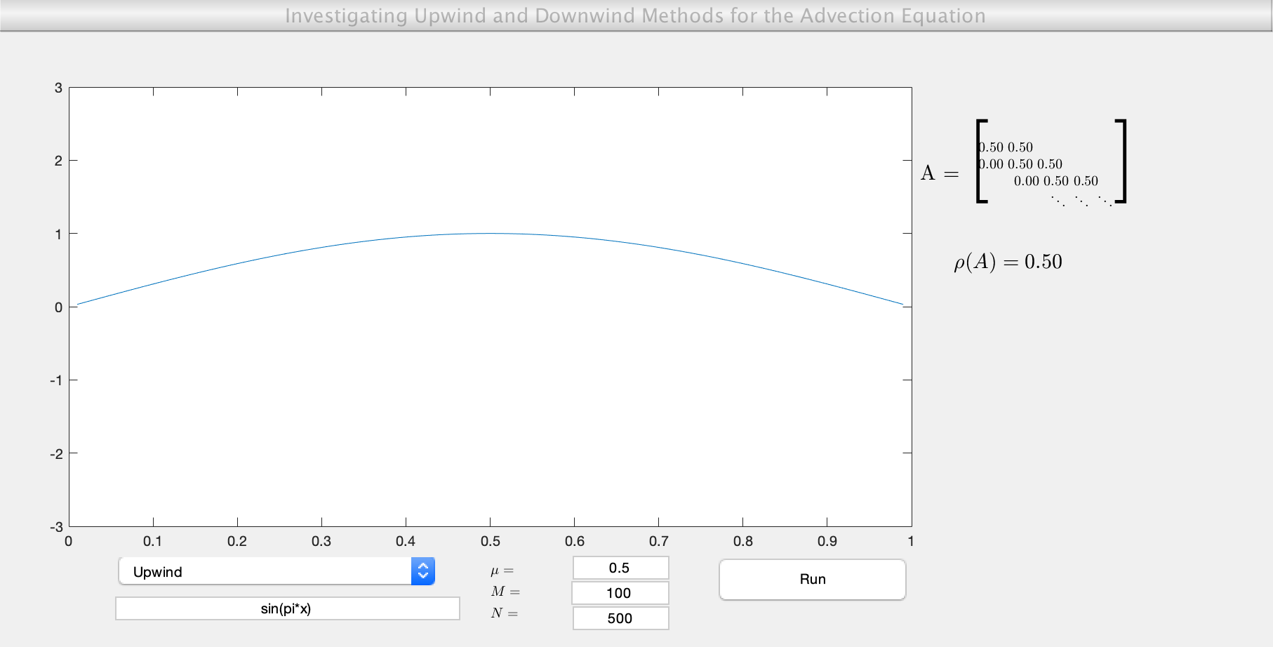
The GUI

Running the downloadable MATLAB code on this page opens a GUI which allows you to vary the method (Upwind vs Downwind) and use different inital condtions). For some methods the GUI will display the matrix which is being used for the calculations. Investigate why the spectral radius and stability region differ for upwinding and downwinding.

advection_gui

The Heaviside Step Function

Perhaps the clearest demonstration of what can go wrong with downwinding is the heaviside step function. The program runs as expected when we use an upwinding method and the step function moves smoothly to the left. However, when we used a downwinding method problems appear immediately from the point of discontinuity. Rather than the points to the left of the jump growing as the wave advances toward them, they remain unchanged. (Afterall, the data from their left remains constant). The points to the right of the discontinuity are receiving their data from the discontinuity, and this causes them to rise sharply as demonstrated in the program.

Wave packet

The function $f(x) = sin(kx)exp(-Kx^2)$ is useful when analysing the advection equation since we can easily see the behaviour of the numerical scheme at a variety of frequencies. The speed at which these waves propagate is a function of their group velocity which varies depending on the frequency and method. In general this will differ from the constant speed demanded by the advection equation, and can indeed be the opposite direction! Some interesting parameters to try:

(Be patient, some of these may take a while to load and calculate on depending on your hardware!)

Code

MathWorks

All files as .zip archive: advection_all.zip

Published with MATLAB® R2017a