Chebyshev Methods for Differential Equations and Example Sheet 2, Question 20
We are already familiar with Fourier spectral methods for differential and partial differential equations. However, there is a significant restriction as to the applicability of spectral methods: spectral convergence depends on both analyticity and periodicity of the problem (including boundary conditions!) So in order to make use of spectral methods in the general case, we need to be more careful...
Contents
Chebyshev expansion and Chebyshev deriviatives
Since the Chebyshev polynomials are a complete orthonormal spanning set on ![$[-1,1]$](chebyshev_eq01893875229900969577.png) we can write
we can write

The coefficients  can be related to Fourier coefficients of
  .
.
Since the  are also polynomials of degree
  , we know that their derivatives are polynomials of degree
  so they must have an expansion in terms of
  . In the Lecture Notes there is a demonstration of how to do this.
How to use this method in practice
MATLAB® represents polynomials as vectors of the coefficients. Taking note of this and using it to represent Chebyshev expansions as vectors in the coefficients, we store:  as
as
f = [1 1.4 0 1 2]';
In order to take deriviatives of  we can use a linear map taking our vector to it's derivative. This vector will have the form:
n = 7;
D = zeros(n);
for i = 1:n
    if mod(i,2) == 1
        D(2*(1:((i-1)/2)),i) = 2*(i-1);
    else
        D(1,i) = i-1;
        D(2*(2:((i)/2))-1,i) = 2*(i-1);
    end
end
D
D =

     0     1     0     3     0     5     0
     0     0     4     0     8     0    12
     0     0     0     6     0    10     0
     0     0     0     0     8     0    12
     0     0     0     0     0    10     0
     0     0     0     0     0     0    12
     0     0     0     0     0     0     0
It is easy to see the structure we expect in this matrix: the first column is all zeros ( ), the other columns have alternate zero and non-zero entries as expected from the forms of the derivatives in the notes.
Solving an equation
We are going to investigate the ODE  on the interval . We can solve this using A-level methods reasonably easily:
  . Let's see how the Chebyshev spectral method works on this problem.
Firstly we can show that the odd coefficients are  and the even coefficients satisfy
  . (Filling in the details of this is Exercise 20, (a) on the example sheet 2.)
Now we want to solve the method by truncating the Chebyshev series expansion of  and solving on a finite domain. We also need to be careful about how we will be treating "ignoring" the odd coefficients.
Ideally, we want to represent our problem as a linear system:  where
where  is the vector formed by taking the Chebyshev expansion of the forcing term
  . In order to ignore the odd terms, we compute
  and then only take out the even rows and columns. This will then act on the subspace we would like to consider. We also need to work out a way to force the linear system to consider the bounday conditions:
  . We can do this by including another row in our matrix and forcing this to equal as well. Therefore our final system will look something like this:
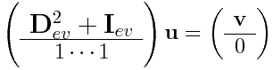
We can set up and solve equations like this very quickly in MATLAB®. One thing to notice about this equation is that we are overconstrained. Therefore when we solve this equation only approximately, via least-squares method, and the lsqlin function of MATLAB®. The following evaluates this method with n=5.
Plots of solution
hold on;
n = 5;
v = zeros(n,1);
v(1) = 1;
u = chebyshev_solv(n,v);
u = pad_ev(u);
x = -1:0.01:1;
subplot(2,1,1); plot(x,evaluate_cheb(u,x),'LineWidth',2); hold on;
subplot(2,1,1); plot(x,1-cos(x)/cos(1),'-o'); hold on;
err = evaluate_cheb(u,x) - (1-cos(x)/cos(1));
subplot(2,1,2); plot(x,err);
hold off;
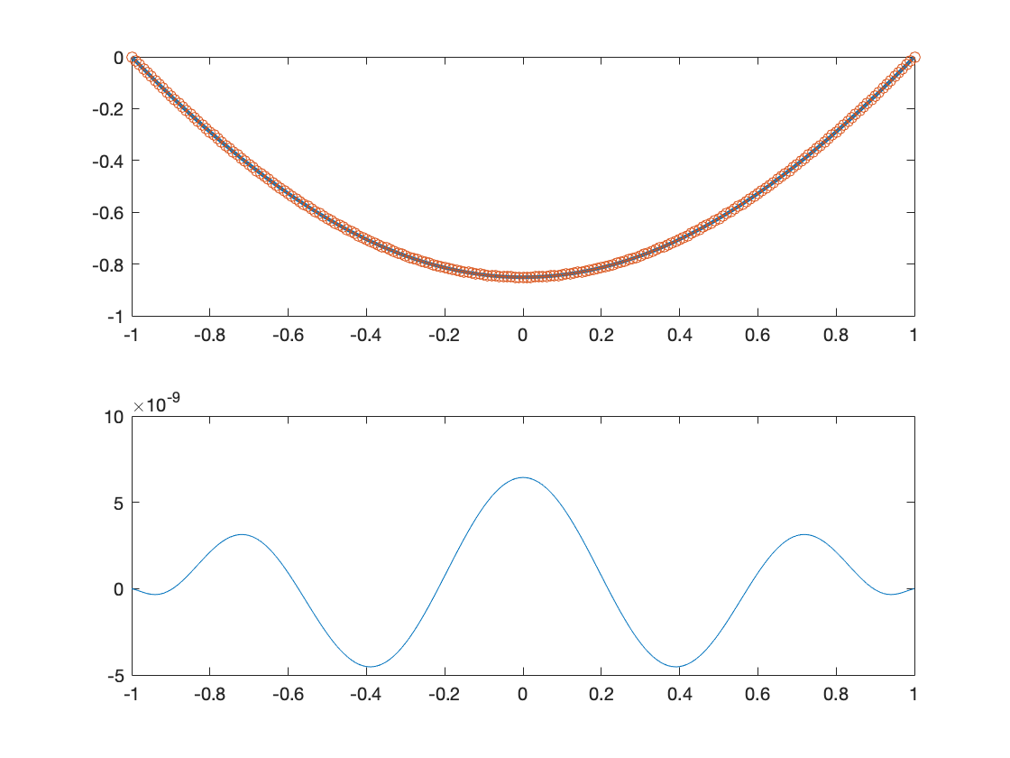
The solution, even for  is very close to the actual solution, illustrating the power of spectral convergence.
Code
See above examples for usage.
- chebyshev_solv.m
- chebyshev_mat.m (Required by chebyshev_solv.m)
- pad_ev.m
- evaluate_cheb.m
All files as .zip archive: chebyshev_all.zip