Stencils and Image Manipulation

Introduction
Review
Stencils as Image Transformations
The GUI
Preset Stencils
Code

Introduction

Stencils are a useful shorthand and calculational tool on grids. For example, the 5-point approximation to $\nabla^2$ from lectures can be represented by the (hopefully increasingly familiar) stencil

laplace5pt = [ 0 1 0; 1 -4 1; 0 1 0];
display(laplace5pt);

laplace5pt =

     0     1     0
     1    -4     1
     0     1     0

Review

Stencils as Image Transformations

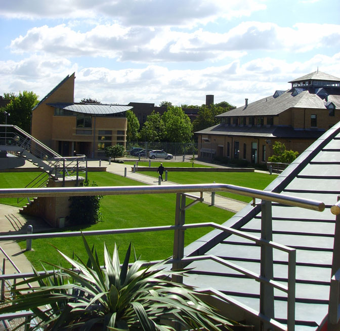
In this unit we explore a few more stencils by using them to represent an image transformation. After all, a digital image in MATLAB is just an array of numbers representing colour values. By applying the stencil to each point of the original image, and storing each result, we produce a new image. Many interesting image transformations can be carried out in this way.

The GUI

Running the downloadable MATLAB code at the bottom of this page starts a Graphical User Interface (GUI):

stencil_demo

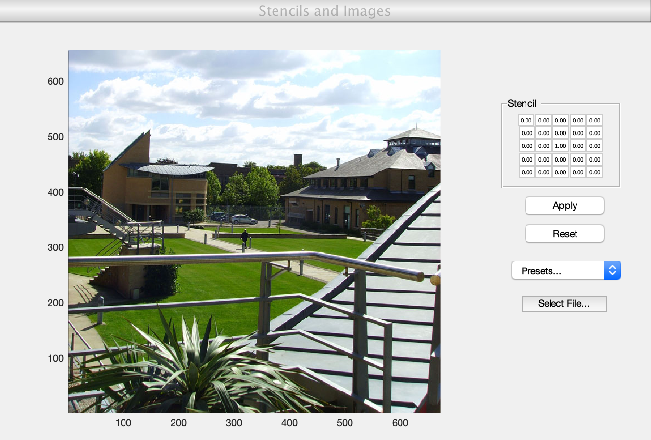
On the right-hand side there is a representation of the stencil

identity = zeros(5,5);
identity(3,3)=1;
display(identity);

identity =

     0     0     0     0     0
     0     0     0     0     0
     0     0     1     0     0
     0     0     0     0     0
     0     0     0     0     0

This stencil is not very exciting; it just represents the identity transformation which leaves the image completely unchanged.

You can apply a stencil of your choice by entering it into the text boxes and clicking the 'Apply' button. To return to the orignal image after a series of stencils have been applied, press the 'Reset' button.

Preset Stencils

Notice the popup menu entitled 'Preset Stencils...'; here we have included some standard stencils so that you don't need to type them in yourself. These are explained in more detail below.

Note that we take $h=1$ (the grid spacing is 1 pixel) in all stencils.

Laplacian (5pt)

This is the 5-point approximation to $\nabla^2$ mentioned in the Introduction:

$\frac{1}{h^2}\times\begin{array}{ccc} & 1 & \\ 1 & -4 & 1\\ & 1 & \\ \end{array}$

Laplacian (9pt)

This is a 9-point approximation to $\nabla^2$ with stencil:

$\frac{1}{6h^2} \times \begin{array}{ccc} 1 & 4 & 1 \\ 4 & -20 & 4\\ 1 & 4 & 1 \\ \end{array}$

Biharmonic (13pt)

This is a 13-point approximation to $\nabla^4$ with stencil:

$\frac{1}{h^4} \times \begin{array}{ccccc} & & 1 & & \\ & 2 & -8 & 2 &\\ 1 & -8 & 20 & -8 & 1 \\ & 2 & -8 & 2 & \\ & & 1 & & \end{array}$

Simpson's Rule (9pt)

This is a 9-point approximation to the two-dimensional integral with stencil:

$\frac{h^2}{9} \times \begin{array}{ccc} 1 & 4 & 1 \\ 4 & 16 & 4\\ 1 & 4 & 1 \\ \end{array}$

Gaussian Blur (9pt)

This is a stencil

$\begin{array}{ccc} s_{{-1},{-1}} & s_{{-1},{0}} & s_{{-1},{1}} \\ s_{{0},{-1}} & s_{{0},{0}} & s_{{0},{1}}\\ s_{{1},{-1}} & s_{{1},{0}} & s_{{1},{1}} \\ \end{array}$

with

$s_{i,j}=\frac{1}{\sqrt{2\pi \sigma^2}} \exp \left[ -\frac{1}{2\sigma^2} \left( i^2 + j^2 \right) \right]$

In this case, we take $\sigma = 0.5$ . More information can be found at http://en.wikipedia.org/wiki/Gaussian_blur

Code

stencil_demo.m (Run this)
stencil_demo.fig (Required)
photo1.jpg (Required - test photo)

All files as .zip archive: stencil_all.zip