3 Introducing Riemannian Geometry

We have yet to meet the star of the show. There is one object that we can place on a manifold whose importance dwarfs all others, at least when it comes to understanding gravity. This is the metric.

The existence of a metric brings a whole host of new concepts to the table which, collectively, are called Riemannian geometry. In fact, strictly speaking we will need a slightly different kind of metric for our study of gravity, one which, like the Minkowski metric, has some strange minus signs. This is referred to as Lorentzian Geometry and a slightly better name for this section would be “Introducing Riemannian and Lorentzian Geometry”. However, for our immediate purposes the differences are minor. The novelties of Lorentzian geometry will become more pronounced later in the course when we explore some of the physical consequences such as horizons.

3.1 The Metric

In Section 1, we informally introduced the metric as a way to measure distances between points. It does, indeed, provide this service but it is not its initial purpose. Instead, the metric is an inner product on each vector space $T_{p}(M)$ .

Definition: A metric $g$ is a $(0,2)$ tensor field that is:

•

Symmetric: $g(X,Y)=g(Y,X)$ .
•

Non-Degenerate: If, for any $p\in M$ , $g(X,Y)\big{|}_{p}=0$ for all $Y\in T_{p}(M)$ then $X_{p}=0$ .

With a choice of coordinates, we can write the metric as

\displaystyle g=g_{\mu\nu}(x)\,dx^{\mu}\otimes dx^{\nu}

The object $g$ is often written as a line element $ds^{2}$ and this expression is abbreviated as

\displaystyle ds^{2}=g_{\mu\nu}(x)\,dx^{\mu}dx^{\nu}

This is the form that we saw previously in (1.5). The metric components can extracted by evaluating the metric on a pair of basis elements,

\displaystyle g_{\mu\nu}(x)=g\left(\frac{\partial{}}{\partial{x^{\mu}}},\frac{% \partial{}}{\partial{x^{\nu}}}\right)

The metric $g_{\mu\nu}$ is a symmetric matrix. We can always pick a basis $e_{\mu}$ of each $T_{p}(M)$ so that this matrix is diagonal. The non-degeneracy condition above ensures that none of these diagonal elements vanish. Some are positive, some are negative. Sylvester’s law of inertia is a theorem in algebra which states that the number of positive and negative entries is independent of the choice of basis. (This theorem has nothing to do with inertia. But Sylvester thought that if Newton could have a law of inertia, there should be no reason he couldn’t.) The number of negative entries is called the signature of the metric.

3.1.1 Riemannian Manifolds

For most applications of differential geometry, we are interested in manifolds in which all diagonal entries of the metric are positive. A manifold equipped with such a metric is called a Riemannian manifold. The simplest example is Euclidean space ${\bf R}^{n}$ which, in Cartesian coordinates, is equipped with the metric

\displaystyle g=dx^{1}\otimes dx^{1}+\ldots+dx^{n}\otimes dx^{n}

The components of this metric are simply $g_{\mu\nu}=\delta_{\mu\nu}$ .

A general Riemannian metric gives us a way to measure the length of a vector $X$ at each point,

\displaystyle|X|=\sqrt{g(X,X)}

It also allows us to measure the angle between any two vectors $X$ and $Y$ at each point, using

\displaystyle g(X,Y)=|X||Y|\cos\theta

The metric also gives us a way to measure the distance between two points $p$ and $q$ along a curve in $M$ . The curve is parameterised by $\sigma:[a,b]\rightarrow M$ , with $\sigma(a)=p$ and $\sigma(b)=q$ . The distance is then

\displaystyle{\rm distance}=\int_{a}^{b}dt\ \sqrt{g(X,X)\big{|}_{\sigma(t)}}

where $X$ is a vector field that is tangent to the curve. If the curve has coordinates $x^{\mu}(t)$ , the tangent vector is $X^{\mu}=dx^{\mu}/dt$ , and the distance is

\displaystyle{\rm distance}=\int_{a}^{b}dt\sqrt{g_{\mu\nu}(x)\frac{dx^{\mu}}{% dt}\frac{dx^{\nu}}{dt}}

Importantly, this distance does not depend on the choice of parameterisation of the curve; this is essentially the same calculation that we did in Section 1.2 when showing the reparameterisation invariance of the action for a particle.

3.1.2 Lorentzian Manifolds

For the purposes of general relativity, we will be working with a manifold in which one of the diagonal entries of the metric is negative. A manifold equipped with such a metric is called Lorentzian.

The simplest example of a Lorentzian metric is Minkowski space. This is ${\bf R}^{n}$ equipped with the metric

\displaystyle\eta=-dx^{0}\otimes dx^{0}+dx^{1}\otimes dx^{1}+\ldots+dx^{n-1}% \otimes dx^{n-1}

The components of the Minkowski metric are $\eta_{\mu\nu}={\rm diag}(-1,+1,\ldots,+1)$ . As this example shows, on a Lorentzian manifold we usually take the coordinate index $x^{\mu}$ to run from $0,1,\ldots,n-1$ .

At any point $p$ on a general Lorentzian manifold, it is always possible to find an orthonormal basis $\{e_{\mu}\}$ of $T_{p}(M)$ such that, locally, the metric looks like the Minkowski metric

\displaystyle g_{\mu\nu}\big{|}_{p}=\eta_{\mu\nu}

(3.93)

This fact is closely related to the equivalence principle; we’ll describe the coordinates that allow us to do this in Section 3.3.2.

In fact, if we find one set of coordinates in which the metric looks like Minkowski space at $p$ , it is simple to exhibit other coordinates. Consider a different basis of vector fields related by

\displaystyle\tilde{e}_{\mu}=\Lambda^{\nu}_{\ \mu}e_{\nu}

Then, in this basis the components of the metric are

\displaystyle\tilde{g}_{\mu\nu}=\Lambda^{\rho}_{\ \mu}\Lambda^{\sigma}_{\ \nu}% g_{\rho\sigma}

This leaves the metric in Minkowski form at $p$ if

\displaystyle\eta_{\mu\nu}=\Lambda^{\rho}_{\ \mu}(p)\Lambda^{\sigma}_{\ \nu}(p% )\eta_{\rho\sigma}

(3.94)

This is the defining equation for a Lorentz transformation that we saw previously in (1.15). We see that viewed locally – which here means at a point $p$ – we recover some basic features of special relativity. Note, however, that if we choose coordinates so that the metric takes the form (3.93) at some point $p$ , it will likely differ from the Minkowski metric as we move away from $p$ .

Figure 21: The lightcone at a point

p

, with three different types of tangent vectors.

The fact that, locally, the metric looks like the Minkowski metric means that we can import some ideas from special relativity. At any point $p$ , a vector $X_{p}\in T_{p}(M)$ is said to be timelike if $g(X_{p},X_{p})<0$ , null if $g(X_{p},X_{p})=0$ , and spacelike if $g(X_{p},X_{p})>0$ .

At each point on $M$ , we can then draw lightcones, which are the null tangent vectors at that point. There are both past-directed and future-directed lightcones at each point, as shown in Figure 21. The novelty is that the directions of these lightcones can vary smoothly as we move around the manifold. This specifies the causal structure of spacetime, which determines who can be friends with whom. We’ll see more of this later in the lectures.

We can again use the metric to determine the length of curves. The nature of a curve at a point is inherited from the nature of its tangent vector. A curve is called timelike if its tangent vector is everywhere timelike. In this case, we can again use the metric to measure the distance along the curve between two points $p$ and $q$ . Given a parametrisation $x^{\mu}(t)$ , this distance is,

\displaystyle\tau=\int_{a}^{b}dt\ \sqrt{-g_{\mu\nu}\frac{dx^{\mu}}{dt}\frac{dx% ^{\nu}}{dt}}

This is called the proper time. It is, in fact, something we’ve met before: it is precisely the action (1.28) for a point particle moving in the spacetime with metric $g_{\mu\nu}$ .

3.1.3 The Joys of a Metric

Whether we’re on a Riemannian or Lorentzian manifold, there are a number of bounties that the metric brings.

The Metric as an Isomophism

First, the metric gives us a natural isomorphism between vectors and covectors, $g:T_{p}(M)\rightarrow T_{p}^{\ast}(M)$ for each $p$ , with the one-form constructed from the contraction of $g$ and a vector field $X$ .

In a coordinate basis, we write $X=X^{\mu}\partial_{\mu}$ . This is mapped to a one-form which, because this is a natural isomorphism, we also call $X$ . This notation is less annoying than you might think; in components the one-form is written is as $X=X_{\mu}dx^{\mu}$ . The components are then related by

\displaystyle X_{\mu}=g_{\mu\nu}X^{\nu}

Physicists usually say that we use the metric to lower the index from $X^{\mu}$ to $X_{\mu}$ . But in their heart, they mean “the metric provides a natural isomorphism between a vector space and its dual”.

Because $g$ is non-degenerate, the matrix $g_{\mu\nu}$ is invertible. We denote the inverse as $g^{\mu\nu}$ , with $g^{\mu\nu}g_{\nu\rho}=\delta^{\mu}_{\rho}$ . Here $g^{\mu\nu}$ can be thought of as the components of a symmetric $(2,0)$ tensor $\hat{g}=g^{\mu\nu}\partial_{\mu}\otimes\partial_{\nu}$ . More importantly, the inverse metric allows us to raise the index on a one-form to give us back the original tangent vector,

\displaystyle X^{\mu}=g^{\mu\nu}X_{\nu}

In Euclidean space, with Cartesian coordinates, the metric is simply $g_{\mu\nu}=\delta_{\mu\nu}$ which is so simple it hides the distinction between vectors and one-forms. This is the reason we didn’t notice the difference between these spaces when we were five.

The Volume Form

The metric also gives us a natural volume form on the manifold $M$ . On a Riemannian manifold, this is defined as

\displaystyle v=\sqrt{{\rm det}g_{\mu\nu}}\,dx^{1}\wedge\ldots\wedge dx^{n}

The determinant is usually simply written as $\sqrt{g}=\sqrt{\det g_{\mu\nu}}$ . On a Lorentzian manifold, the determinant is negative and we instead have

\displaystyle v=\sqrt{-g}\,dx^{0}\wedge\ldots\wedge dx^{n-1}

(3.95)

As defined, the volume form looks coordinate dependent. Importantly, it is not. To see this, introduce some rival coordinates $\tilde{x}^{\mu}$ , with

\displaystyle dx^{\mu}=A^{\mu}_{\ \nu}d\tilde{x}^{\nu}\ \ \ {\rm where}\ \ A^{% \mu}_{\ \nu}=\frac{\partial{x^{\mu}}}{\partial{\tilde{x}^{\nu}}}

In the new coordinates, the wedgey part of the volume form becomes

\displaystyle dx^{1}\wedge\ldots\wedge dx^{n}=A^{1}_{\ \mu_{1}}\ldots A^{n}_{% \ \mu_{n}}d\tilde{x}^{\mu_{1}}\wedge\ldots\wedge d\tilde{x}^{\mu_{n}}

We can rearrange the one-forms into the order $d\tilde{x}^{1}\wedge\ldots\wedge d\tilde{x}^{n}$ . We pay a price of $+$ or $-1$ depending on whether $\{\mu_{1},\ldots,\mu_{n}\}$ is an even or odd permutation of $\{1,\ldots,n\}$ . Since we’re summing over all indices, this is the same as summing over all permutations $\pi$ of $\{1,\ldots,n\}$ , and we have

	$\displaystyle dx^{1}\wedge\ldots\wedge dx^{n}$	$\displaystyle=$	$\displaystyle\sum_{\mbox{perms\ $\pi$}}\mbox{sign($\pi$)}\,A^{1}_{\pi(1)}% \ldots A^{n}_{\pi(n)}d\tilde{x}^{1}\wedge\ldots\wedge d\tilde{x}^{n}$
		$\displaystyle=$	$\displaystyle{\rm det}(A)\,d\tilde{x}^{1}\wedge\ldots\wedge d\tilde{x}^{n}$

where $\det(A)>0$ if the change of coordinates preserves the orientation. This factor of $\det(A)$ is the usual Jacobian factor that one finds when changing the measure in an integral.

Meanwhile, the metric components transform as

\displaystyle{g}_{\mu\nu}=\frac{\partial{\tilde{x}^{\rho}}}{\partial{x^{\mu}}}% \frac{\partial{\tilde{x}^{\sigma}}}{\partial{x^{\nu}}}\tilde{g}_{\rho\sigma}=(% A^{-1})^{\rho}_{\ \mu}(A^{-1})^{\sigma}_{\ \nu}\tilde{g}_{\rho\sigma}

and so the determinant becomes

\displaystyle\det g_{\mu\nu}=(\det\,A^{-1})^{2}\det\tilde{g}_{\mu\nu}=\frac{% \det\tilde{g}_{\mu\nu}}{(\det A)^{2}}

We see that the factors of $\det A$ cancel, and we can equally write the volume form as

\displaystyle v=\sqrt{|\tilde{g}|}\,d\tilde{x}^{1}\wedge\ldots\wedge d\tilde{x% }^{n}

The volume form (3.95) may look more familiar if we write it as

\displaystyle v=\frac{1}{n!}v_{\mu_{1}\ldots\mu_{n}}dx^{\mu_{1}}\wedge\ldots% \wedge dx^{\mu_{n}}

Here the components $v_{\mu_{1}\ldots\mu_{n}}$ are given in terms of the totally anti-symmetric object $\epsilon_{\mu_{1}\ldots\mu_{n}}$ with $\epsilon_{1\ldots n}=+1$ and other components determined by the sign of the permutation,

\displaystyle v_{\mu_{1}\ldots\mu_{n}}=\sqrt{|g|}\,\epsilon_{\mu_{1}\ldots\mu_% {n}}

(3.96)

Note that $v_{\mu_{1}\ldots\mu_{n}}$ is a tensor, which means that $\epsilon_{\mu_{1}\ldots\mu_{n}}$ can’t quite be a tensor: instead, it is a tensor divided by $\sqrt{|g|}$ . It is sometimes said to be a tensor density. The anti-symmetric tensor density arises in many places in physics. In all cases, it should be viewed as a volume form on the manifold. (In nearly all cases, this volume form arises from a metric as here.)

As with other tensors, we can use the metric to raise the indices and construct the volume form with all indices up

\displaystyle v^{\mu_{1}\ldots\mu_{n}}=g^{\mu_{1}\nu_{1}}\ldots g^{\mu_{n}\nu_% {n}}v_{\nu_{1}\ldots\nu_{n}}=\pm\frac{1}{\sqrt{|g|}}\epsilon^{\mu_{1}\ldots\mu% _{n}}

where we get a $+$ sign for a Riemannian manifold, and a $-$ sign for a Lorentzian manifold. Here $\epsilon^{\mu_{1}\ldots\mu_{n}}$ is again a totally anti-symmetric tensor density with $\epsilon^{1\ldots n}=+1$ . Note, however, that while we raise the indices on $v_{\mu_{1}\ldots\mu_{n}}$ using the metric, this statement doesn’t quite hold for $\epsilon_{\mu_{1}\ldots\mu_{n}}$ which takes values 1 or 0 regardless of whether the indices are all down or all up. This reflects the fact that it is a tensor density, rather than a genuine tensor.

The existence of a natural volume form means that, given a metric, we can integrate any function $f$ over the manifold. We will sometimes write this as

\displaystyle\int_{M}fv=\int_{M}d^{n}x\ \sqrt{\pm g}f

The metric $\sqrt{\pm g}$ provides a measure on the manifold that tells us what regions of the manifold are weighted more strongly than the others in the integral.

The Hodge Dual

On an oriented manifold $M$ , we can use the totally anti-symmetric tensor $\epsilon_{\mu_{1},\ldots,\mu_{n}}$ to define a map which takes a $p$ -form $\omega\in\Lambda^{p}(M)$ to an $(n-p)$ -form, denoted $(\star\,\omega)\in\Lambda^{n-p}(M)$ , defined by

\displaystyle(\star\,\omega)_{\mu_{1}\ldots\mu_{n-p}}=\frac{1}{p!}\sqrt{|g|}\,% \epsilon_{\mu_{1}\ldots\mu_{n-p}\nu_{1}\ldots\nu_{p}}\omega^{\nu_{1}\ldots\nu_% {p}}

(3.97)

This map is called the Hodge dual. It is independent of the choice of coordinates.

It’s not hard to check that,

\displaystyle\star\,(\star\,\omega)=\pm(-1)^{p(n-p)}\omega

(3.98)

where the $+$ sign holds for Riemannian manifolds and the $-$ sign for Lorentzian manifolds. (To prove this, it’s useful to first show that $v^{\mu_{1}\ldots\mu_{p}\rho_{1}\ldots\rho_{n-p}}v_{\nu_{1}\ldots\nu_{p}\rho_{1% }\ldots\rho_{n-p}}=\pm p!(n-p)!\delta^{\mu_{1}}_{[\nu_{1}}\ldots\delta^{\mu_{p% }}_{\nu_{p}]}$ , again with the $\pm$ sign for Riemannian/Lorentzian manifolds.)

It’s worth returning to some high school physics and viewing it through the lens of our new tools. We are very used to taking two vectors in ${\bf R}^{3}$ , say ${\bf a}$ and ${\bf b}$ , and taking the cross-product to find a third vector

\displaystyle{\bf a}\times{\bf b}={\bf c}

In fact, we really have objects that live in three different spaces here, related by the Euclidean metric $\delta_{\mu\nu}$ . First we use this metric to relate the vectors to one-forms. The cross-product is then really a wedge product which gives us back a 2-form. We then use the metric twice more, once to turn the two-form back into a one-form using the Hodge dual, and again to turn the one-form into a vector. Of course, none of these subtleties bothered us when we were 15. But when we start thinking about curved manifolds, with a non-trivial metric, these distinctions become important.

The Hodge dual allows us to define an inner product on each $\Lambda^{p}(M)$ . If $\omega,\eta\in\Lambda^{p}(M)$ , we define

\displaystyle\langle\eta,\omega\rangle=\int_{M}\eta\wedge\star\,\omega

which makes sense because $\star\,\omega\in\Lambda^{n-p}(M)$ and so $\eta\wedge\star\,\omega$ is a top form that can be integrated over the manifold.

With such an inner product in place, we can also start to play the kind of games that are familiar from quantum mechanics and look at operators on $\Lambda^{p}(M)$ and their adjoints. The one operator that we have introduced on the space of forms is the exterior derivative, defined in Section 2.4.1. Its adjoint is defined by the following result:

Claim: For $\omega\in\Lambda^{p}(M)$ and $\alpha\in\Lambda^{p-1}(M)$ ,

\displaystyle\langle d\alpha,\omega\rangle=\langle\alpha,d^{\dagger}\omega\rangle

(3.99)

where the adjoint operator $d^{\dagger}:\Lambda^{p}(M)\rightarrow\Lambda^{p-1}(M)$ is given by

\displaystyle d^{\dagger}=\pm(-1)^{np+n-1}\star\,d\,\star

with, again, the $\pm$ sign for Riemannian/Lorentzian manifolds respectively.

Proof: This is simply the statement of integration-by-parts for forms. On a closed manifold $M$ , Stokes’ theorem tells us that

\displaystyle 0=\int_{M}d(\alpha\wedge\star\,\omega)=\int_{M}d\alpha\wedge% \star\,\omega+(-1)^{p-1}\alpha\wedge d\,\star\,\omega

The first term is simply $\langle d\alpha,\omega\rangle$ . The second term also takes the form of an inner product which, up to a sign, is proportional to $\langle\alpha,\star\,d\,\star\,\omega\rangle$ . To determine the sign, note that $d\,\star\omega\in\Lambda^{n-p+1}(M)$ so, using (3.98), we have $\star\,\star\,d\star\,\omega=\pm(-1)^{(n-p+1)(p-1)}d\,\star\,\omega$ . Putting this together gives

\displaystyle\langle d\alpha,\omega\rangle=\pm(-1)^{np+n-1}\langle\alpha,\star% \,d\star\,\omega\rangle

as promised. $\Box$

3.1.4 A Sniff of Hodge Theory

We can combine $d$ and $d^{\dagger}$ to construct the Laplacian, $\bigtriangleup:\Lambda^{p}(M)\rightarrow\Lambda^{p}(M)$ , defined as

\displaystyle\bigtriangleup=(d+d^{\dagger})^{2}=dd^{\dagger}+d^{\dagger}d

where the second equality follows because $d^{2}=d^{\dagger\,2}=0$ . The Laplacian can be defined on both Riemannian manifolds, where it is positive definite, and Lorentzian manifolds. Here we restrict our discussion to Riemannian manifolds.

Acting on functions $f$ , we have $d^{\dagger}f=0$ (because $\star\,f$ is a top form so $d\,\star\,f=0$ ). That leaves us with,

$\displaystyle\bigtriangleup(f)$	$\displaystyle=$	$\displaystyle-\star\,d\,\star\left(\partial_{\mu}f\,dx^{\mu}\right)$
	$\displaystyle=$	$\displaystyle-\frac{1}{(n-1)!}\star\,d\,\left((\partial_{\mu}f)g^{\mu\nu}\sqrt% {\|g\|}\,\epsilon_{\nu\rho_{1}\ldots\rho_{n-1}}dx^{\rho_{1}}\wedge\ldots\wedge dx% ^{\rho_{n-1}}\right)$
	$\displaystyle=$	$\displaystyle-\frac{1}{(n-1)!}\star\,\partial_{\sigma}\left(\sqrt{\|g\|}g^{\mu% \nu}\partial_{\mu}f\right)\epsilon_{\nu\rho_{1}\ldots\rho_{n-1}}dx^{\sigma}% \wedge dx^{\rho_{1}}\wedge\ldots\wedge dx^{\rho_{n-1}}$
	$\displaystyle=$	$\displaystyle-\star\,\partial_{\nu}\left(\sqrt{\|g\|}g^{\mu\nu}\partial_{\mu}f% \right)dx^{1}\wedge\ldots\wedge dx^{n}$
	$\displaystyle=$	$\displaystyle-\frac{1}{\sqrt{\|g\|}}\partial_{\nu}\left(\sqrt{\|g\|}g^{\mu\nu}% \partial_{\mu}f\right)$

This form of the Laplacian, acting on functions, appears fairly often in applications of differential geometry.

There is a particularly nice story involving $p$ -forms $\gamma$ that obey

\displaystyle\bigtriangleup\gamma=0

Such forms are said to be harmonic. An harmonic form is necessarily closed, meaning $d\gamma=0$ , and co-closed, meaning $d^{\dagger}\gamma=0$ . This follows by writing

\displaystyle\langle\gamma,\bigtriangleup\gamma\rangle=\langle d\gamma,d\gamma% \rangle+\langle d^{\dagger}\gamma,d^{\dagger}\gamma\rangle=0

and noting that the inner product is positive-definite.

There are some rather pretty facts that relate the existence of harmonic forms to de Rham cohomology. The space of harmonic $p$ -forms on a manifold $M$ is denoted ${\rm Harm}^{p}(M)$ . First, the Hodge decomposition theorem, which we state without proof: any $p$ -form $\omega$ on a compact, Riemannian manifold can be uniquely decomposed as

\displaystyle\omega=d\alpha+d^{\dagger}\beta+\gamma

where $\alpha\in\Lambda^{p-1}(M)$ and $\beta\in\Lambda^{p+1}(M)$ and $\gamma\in{\rm Harm}^{p}(M)$ . This result can then be used to prove:

Hodge’s Theorem: There is an isomorphism

\displaystyle{\rm Harm}^{p}(M)\cong H^{p}(M)

where $H^{p}(M)$ is the de Rham cohomology group introduced in Section 2.4.3. In particular, the Betti numbers can be computed by counting the number of linearly independent harmonic forms,

\displaystyle B_{p}={\rm dim}\ {\rm Harm}^{p}(M)

Proof: First, let’s show that any harmonic form $\gamma$ provides a representative of $H^{p}(M)$ . As we saw above, any harmonic $p$ -form is closed, $d\gamma=0$ , so $\gamma\in Z^{p}(M)$ . But the unique nature of the Hodge decomposition tells us that $\gamma\neq d\beta$ for some $\beta$ .

Next, we need to show that any equivalence class $[\omega]\in H^{p}(M)$ can be represented by a harmonic form. We decompose $\omega=d\alpha+d^{\dagger}\beta+\gamma$ . By definition $[\omega]\in H^{p}(M)$ means that $d\omega=0$ so we have

\displaystyle 0=\langle d\omega,\beta\rangle=\langle\omega,d^{\dagger}\beta% \rangle=\langle d\alpha+d^{\dagger}\beta+\gamma,d^{\dagger}\beta\rangle=% \langle d^{\dagger}\beta,d^{\dagger}\beta\rangle

where, in the final step, we “integrated by parts” and used the fact that $dd\alpha=d\gamma=0$ . Because the inner product is positive definite, we must have $d^{\dagger}\beta=0$ and, hence, $\omega=\gamma+d\alpha$ . Any other representative $\tilde{\omega}\sim\omega$ of $[\omega]\in H^{p}(M)$ differs by $\tilde{\omega}=\omega+d\eta$ and so, by the Hodge decomposition, is associated to the same harmonic form $\gamma$ . $\Box$

3.2 Connections and Curvature

We’ve already met one version of differentiation in these lectures. A vector field $X$ is, at heart, a differential operator and provides a way to differentiate a function $f$ . We write this simply as $X(f)$ .

As we saw previously, differentiating higher tensor fields is a little more tricky because it requires us to subtract tensor fields at different points. Yet tensors evaluated at different points live in different vector spaces, and it only makes sense to subtract these objects if we can first find a way to map one vector space into the other. In Section 2.2.4, we used the flow generated by $X$ as a way to perform this mapping, resulting in the idea of the Lie derivative ${\cal L}_{X}$ .

There is, however, a different way to take derivatives, one which ultimately will prove more useful. The derivative is again associated to a vector field $X$ . However, this time we introduce a different object, known as a connection to map the vector spaces at one point to the vector spaces at another. The result is an object, distinct from the Lie derivative, called the covariant derivative.

3.2.1 The Covariant Derivative

A connection is a map $\nabla:\mathfrak{X}(M)\times\mathfrak{X}(M)\rightarrow\mathfrak{X}(M)$ . We usually write this as $\nabla(X,Y)=\nabla_{X}Y$ and the object $\nabla_{X}$ is called the covariant derivative. It satisfies the following properties for all vector fields $X$ , $Y$ and $Z$ ,

•

$\nabla_{X}(Y+Z)=\nabla_{X}Y+\nabla_{X}Z$
•

$\nabla_{(fX+gY)}Z=f\nabla_{X}Z+g\nabla_{Y}Z$ for all functions $f, g$ .
•

$\nabla_{X}(fY)=f\nabla_{X}Y+(\nabla_{X}f)Y$ where we define $\nabla_{X}f=X(f)$

The covariant derivative endows the manifold with more structure. To elucidate this, we can evaluate the connection in a basis $\{e_{\mu}\}$ of $\mathfrak{X}(M)$ . We can always express this as

\displaystyle\nabla_{e_{\rho}}e_{\nu}=\Gamma^{\mu}_{\,\rho\nu}e_{\mu}

(3.100)

with $\Gamma^{\mu}_{\rho\nu}$ the components of the connection. It is no coincidence that these are denoted by the same greek letter that we used for the Christoffel symbols in Section 1. However, for now, you should not conflate the two; we’ll see the relationship between them in Section 3.2.3.

The name “connection” suggests that $\nabla$ , or its components $\Gamma^{\mu}_{\,\nu\rho}$ , connect things. Indeed they do. We will show in Section 3.3 that the connection provides a map from the tangent space $T_{p}(M)$ to the tangent space at any other point $T_{q}(M)$ . This is what allows the connection to act as a derivative.

We will use the notation

\displaystyle\nabla_{\mu}=\nabla_{e_{\mu}}

This makes the covariant derivative $\nabla_{\mu}$ look similar to a partial derivative. Using the properties of the connection, we can write a general covariant derivative of a vector field as

$\displaystyle\nabla_{X}Y$	$\displaystyle=$	$\displaystyle\nabla_{X}(Y^{\mu}e_{\mu})$
	$\displaystyle=$	$\displaystyle X(Y^{\mu})e_{\mu}+Y^{\mu}\nabla_{X}e_{\mu}$
	$\displaystyle=$	$\displaystyle X^{\nu}e_{\nu}(Y^{\mu})e_{\mu}+X^{\nu}Y^{\mu}\nabla_{\nu}e_{\mu}$
	$\displaystyle=$	$\displaystyle X^{\nu}\left(e_{\nu}(Y^{\mu})+\Gamma_{\,\nu\rho}^{\mu}Y^{\rho}% \right)e_{\mu}$

The fact that we can strip off the overall factor of $X^{\nu}$ means that it makes sense to write the components of the covariant derivative as

\displaystyle\nabla_{\nu}Y=(e_{\nu}(Y^{\mu})+\Gamma^{\mu}_{\,\nu\rho}Y^{\rho})% e_{\mu}

Or, in components,

\displaystyle(\nabla_{\nu}Y)^{\mu}=e_{\nu}(Y^{\mu})+\Gamma^{\mu}_{\,\nu\rho}Y^% {\rho}

(3.101)

Note that the covariant derivative coincides with the Lie derivative on functions, $\nabla_{X}f={\cal L}_{X}f=X(f)$ . It also coincides with the old-fashioned partial derivative: $\nabla_{\mu}f=\partial_{\mu}f$ . However, its action on vector fields differs. In particular, the Lie derivative ${\cal L}_{X}Y=[X,Y]$ depends on both $X$ and the first derivative of $X$ while, as we have seen above, the covariant derivative depends only on $X$ . This is the property that allows us to write $\nabla_{X}=X^{\nu}\nabla_{\nu}$ and think of $\nabla_{\mu}$ as an operator in its own right. In contrast, there is no way to write “ ${\cal L}_{X}=X^{\mu}{\cal L}_{\mu}$ ”. While the Lie derivative has its uses, the ability to define $\nabla_{\mu}$ means that this is best viewed as the natural generalisation of the partial derivative to curved space.

Differentiation as Punctuation

In a coordinate basis, in which $e_{\mu}=\partial_{\mu}$ , the covariant derivative (3.101) becomes

\displaystyle(\nabla_{\nu}Y)^{\mu}=\partial_{\nu}Y^{\mu}+\Gamma^{\mu}_{\,\nu% \rho}Y^{\rho}

(3.102)

We will differentiate often. To save ink, we use the sloppy, and sometimes confusing, notation

\displaystyle(\nabla_{\nu}Y)^{\mu}=\nabla_{\nu}Y^{\mu}

This means, in particular, that $\nabla_{\nu}Y^{\mu}$ is the $\mu^{\rm th}$ component of $\nabla_{\nu}Y$ , rather than the differentiation of the function $Y^{\mu}$ .

Covariant differentiation is sometimes denoted using a semi-colon

\displaystyle\nabla_{\nu}Y^{\mu}={Y^{\mu}}_{;\nu}

In this convention, the partial derivative is denoted using a mere comma, $\partial_{\mu}Y^{\nu}={Y^{\nu}}_{,\mu}$ . The expression (3.102) then reads

\displaystyle{Y^{\mu}}_{;\nu}={Y^{\mu}}_{,\nu}+\Gamma^{\mu}_{\,\nu\rho}Y^{\rho}

I’m proud to say that we won’t adopt the “semi-colon = differentiation” notation in these lectures. Because it’s stupid.

The Connection is Not a Tensor

The $\Gamma^{\mu}_{\,\rho\nu}$ defining the connection are not components of a tensor. We can see this immediately from the definition $\nabla(X,fY)=\nabla_{X}(fY)=f\nabla_{X}Y+(X(f))Y$ . This is not linear in the second argument, which is one of the requirements of a tensor.

To illustrate this, we can ask what the connection looks like in a different basis,

\displaystyle\tilde{e}_{\nu}=A^{\mu}_{\ \nu}e_{\mu}

(3.103)

for some invertible matrix $A$ . If $e_{\mu}$ and $\tilde{e}_{\mu}$ are both coordinate bases, then

\displaystyle A^{\mu}_{\ \nu}=\frac{\partial{x^{\mu}}}{\partial{\tilde{x}^{\nu% }}}

We know from (2.78) that the components of a $(1,2)$ tensor transform as

\displaystyle\tilde{T}^{\mu}_{\ \,\nu\rho}=(A^{-1})^{\mu}_{\ \tau}A^{\lambda}_% {\ \nu}A^{\sigma}_{\ \rho}{T^{\tau}}_{\lambda\sigma}

(3.104)

We can now compare this to the transformation of the connection components $\Gamma^{\mu}_{\rho\nu}$ . In the basis $\tilde{e}_{\mu}$ , we have

\displaystyle\nabla_{\tilde{e}_{\rho}}\tilde{e}_{\nu}=\tilde{\Gamma}_{\,\rho% \nu}^{\mu}\tilde{e}_{\mu}

Substituting in the transformation (3.103), we have

\displaystyle\tilde{\Gamma}_{\,\rho\nu}^{\mu}\tilde{e}_{\mu}=\nabla_{(A^{% \sigma}_{\ \rho}e_{\sigma})}(A^{\lambda}_{\ \nu}e_{\lambda})=A^{\sigma}_{\ % \rho}\nabla_{e_{\sigma}}(A^{\lambda}_{\ \nu}e_{\lambda})=A^{\sigma}_{\ \rho}A^% {\lambda}_{\ \nu}\Gamma^{\tau}_{\,\sigma\lambda}e_{\tau}+A^{\sigma}_{\ \rho}e_% {\lambda}\partial_{\sigma}A^{\lambda}_{\ \nu}

We can write this as

	$\displaystyle\tilde{\Gamma}_{\,\rho\nu}^{\mu}\tilde{e}_{\mu}$	$\displaystyle=$	$\displaystyle\left(A^{\sigma}_{\ \rho}A^{\lambda}_{\ \nu}\Gamma^{\tau}_{\,% \sigma\lambda}+A^{\sigma}_{\ \rho}\partial_{\sigma}A^{\tau}_{\ \nu}\right)e_{\tau}$
		$\displaystyle=$	$\displaystyle\left(A^{\sigma}_{\ \rho}A^{\lambda}_{\ \nu}\Gamma^{\tau}_{\,% \sigma\lambda}+A^{\sigma}_{\ \rho}\partial_{\sigma}A^{\tau}_{\ \nu}\right)(A^{% -1})^{\mu}_{\ \tau}\tilde{e}_{\mu}$

Stripping off the basis vectors $\tilde{e}_{\mu}$ , we see that the components of the connection transform as

\displaystyle\tilde{\Gamma}_{\,\rho\nu}^{\mu}=(A^{-1})^{\mu}_{\ \tau}A^{\sigma% }_{\ \rho}A^{\lambda}_{\ \nu}\Gamma^{\tau}_{\,\sigma\lambda}+(A^{-1})^{\mu}_{% \ \tau}A^{\sigma}_{\ \rho}\partial_{\sigma}A^{\tau}_{\ \nu}

(3.105)

The first term coincides with the transformation of a tensor (3.104). But the second term, which is independent of $\Gamma$ , but instead depends on $\partial A$ , is novel. This is the characteristic transformation property of a connection.

Differentiating Other Tensors

We can use the Leibnizarity of the covariant derivative to extend its action to any tensor field. It’s best to illustrate this with an example.

Consider a one-form $\omega$ . If we differentiate $\omega$ , we will get another one-form $\nabla_{X}\omega$ which, like any one-form, is defined by its action on vector fields $Y\in\mathfrak{X}(M)$ . To construct this, we will insist that the connection obeys the Leibnizarity in the modified sense that

\displaystyle\nabla_{X}(\omega(Y))=(\nabla_{X}\omega)(Y)+\omega(\nabla_{X}Y)

But $\omega(Y)$ is simply a function, which means that we can also write this as

\displaystyle\nabla_{X}(\omega(Y))=X(\omega(Y))

Putting these together gives

\displaystyle(\nabla_{X}\omega)(Y)=X(\omega(Y))-\omega(\nabla_{X}Y)

In coordinates, we have

	$\displaystyle X^{\mu}(\nabla_{\mu}\omega)_{\nu}Y^{\nu}$	$\displaystyle=$	$\displaystyle X^{\mu}\partial_{\mu}(\omega_{\nu}Y^{\nu})-\omega_{\nu}X^{\mu}(% \partial_{\mu}Y^{\nu}+\Gamma_{\,\mu\rho}^{\nu}Y^{\rho})$
		$\displaystyle=$	$\displaystyle X^{\mu}(\partial_{\mu}\omega_{\rho}-\Gamma^{\nu}_{\,\mu\rho}% \omega_{\nu})Y^{\rho}$

where, crucially, the $\partial Y$ terms cancel in going from the first to the second line. This means that the overall result is linear in $Y$ and we may define $\nabla_{X}\omega$ without reference to the vector field $Y$ on which is acts. In components, we have

\displaystyle(\nabla_{\mu}\omega)_{\rho}=\partial_{\mu}\omega_{\rho}-\Gamma_{% \,\mu\rho}^{\nu}\omega_{\nu}

As for vector fields, we also write this as

\displaystyle(\nabla_{\mu}\omega)_{\rho}\equiv\nabla_{\mu}\omega_{\rho}\equiv% \omega_{\rho;\mu}=\omega_{\rho,\mu}-\Gamma_{\,\mu\rho}^{\nu}\omega_{\nu}

This kind of argument can be extended to a general tensor field of rank $(p,q)$ , where the covariant derivative is defined by,

	$\displaystyle{T^{\mu_{1}\ldots\mu_{p}}}_{\nu_{1}\ldots\nu_{q};\rho}$	$\displaystyle=$	$\displaystyle{T^{\mu_{1}\ldots\mu_{p}}}_{\nu_{1}\ldots\nu_{q},\rho}+\Gamma^{% \mu_{1}}_{\,\rho\sigma}{T^{\sigma\mu_{2}\ldots\mu_{p}}}_{\nu_{1}\ldots\nu_{q}}% +\ldots+\Gamma^{\mu_{p}}_{\,\rho\sigma}{T^{\mu_{1}\ldots\mu_{p-1}\sigma}}_{\nu% _{1}\ldots\nu_{q}}$
			$\displaystyle\ \ \ \ \ -\Gamma^{\sigma}_{\,\rho\nu_{1}}{T^{\mu_{1}\ldots\mu_{p% }}}_{\sigma\nu_{2}\ldots\nu_{q}}-\ldots-\Gamma^{\sigma}_{\,\rho\nu_{q}}{T^{\mu% _{1}\ldots\mu_{p}}}_{\nu_{1}\ldots\nu_{q-1}\sigma}$

The pattern is clear: for every upper index $\mu$ we get a $+\Gamma T$ term, while for every lower index we get a $-\Gamma T$ term.

Now that we can differentiate tensors, we will also need to extend our punctuation notation slightly. If more than two subscripts follow a semi-colon (or, indeed, a comma) then we differentiate respect to both, doing the one on the left first. So, for example, ${X^{\mu}}_{;\nu\rho}=\nabla_{\rho}\nabla_{\nu}X^{\mu}$ .

3.2.2 Torsion and Curvature

Even though the connection is not a tensor, we can use it to construct two tensors. The first is a rank $(1,2)$ tensor $T$ known as torsion. It is defined to act on $X,Y\in\mathfrak{X}(M)$ and $\omega\in\Lambda^{1}(M)$ by

\displaystyle T(\omega;X,Y)=\omega(\nabla_{X}Y-\nabla_{Y}X-[X,Y])

The other is a rank $(1,3)$ tensor $R$ , known as curvature. It acts on $X,Y,Z\in\mathfrak{X}(M)$ and $\omega\in\Lambda^{1}(M)$ by

\displaystyle R(\omega;X,Y,Z)=\omega(\nabla_{X}\nabla_{Y}Z-\nabla_{Y}\nabla_{X% }Z-\nabla_{[X,Y]}Z)

The curvature tensor is also called the Riemann tensor.

Alternatively, we could think of torsion as a map $T:\mathfrak{X}(M)\times\mathfrak{X}(M)\rightarrow\mathfrak{X}(M)$ , defined by

\displaystyle T(X,Y)=\nabla_{X}Y-\nabla_{Y}X-[X,Y]

Similarly, the curvature $R$ can be viewed as a map from $\mathfrak{X}(M)\times\mathfrak{X}(M)$ to a differential operator acting on $\mathfrak{X}(M)$ ,

\displaystyle R(X,Y)=\nabla_{X}\nabla_{Y}-\nabla_{Y}\nabla_{X}-\nabla_{[X,Y]}

(3.106)

Checking Linearity

To demonstrate that $T$ and $R$ are indeed tensors, we need to show that they are linear in all arguments. Linearity in $\omega$ is straightforward. For the others, there are some small calculations to do. For example, we must show that $T(\omega;fX,Y)=fT(\omega;X,Y)$ . To see this, we just run through the definitions of the various objects,

\displaystyle T(\omega;fX,Y)=\omega(\nabla_{fX}Y-\nabla_{Y}(fX)-[fX,Y])

We then use $\nabla_{fX}Y=f\nabla_{X}Y$ and $\nabla_{Y}(fX)=f\nabla_{Y}X+Y(f)\,X$ and $[fX,Y]=f[X,Y]-Y(f)X$ . The two $Y(f)X$ terms cancel, leaving us with

	$\displaystyle T(\omega;fX,Y)$	$\displaystyle=$	$\displaystyle f\omega(\nabla_{X}Y-\nabla_{Y}X-[X,Y])$
		$\displaystyle=$	$\displaystyle fT(\omega;X,Y)$

Similarly, for the curvature tensor we have

$\displaystyle R(\omega;fX,Y,Z)$	$\displaystyle=$	$\displaystyle\omega(\nabla_{fX}\nabla_{Y}Z-\nabla_{Y}\nabla_{fX}Z-\nabla_{[fX,% Y]}Z$
	$\displaystyle=$	$\displaystyle\omega(f\nabla_{X}\nabla_{Y}Z-\nabla_{Y}(f\nabla_{X}Z)-\nabla_{(f% [X,Y]-Y(f)X)}Z)$
	$\displaystyle=$	$\displaystyle\omega(f\nabla_{X}\nabla_{Y}Z-f\nabla_{Y}\nabla_{X}Z-Y(f)\nabla_{% X}Z-\nabla_{f[X,Y]}Z+\nabla_{Y(f)X}Z)$
	$\displaystyle=$	$\displaystyle\omega(f\nabla_{X}\nabla_{Y}Z-f\nabla_{Y}\nabla_{X}Z-Y(f)\nabla_{% X}Z-f\nabla_{[X,Y]}Z+Y(f)\nabla_{X}Z)$
	$\displaystyle=$	$\displaystyle f\omega(\nabla_{X}\nabla_{Y}Z-\nabla_{Y}\nabla_{X}Z-\nabla_{[X,Y% ]}Z)$
	$\displaystyle=$	$\displaystyle fR(\omega;X,Y,Z)$

Linearity in $Y$ follows from linearity in $X$ . But we still need to check linearity in $Z$ ,

$\displaystyle R(\omega;X,Y,fZ)$	$\displaystyle=$	$\displaystyle\omega(\nabla_{X}\nabla_{Y}(fZ)-\nabla_{Y}\nabla_{X}(fZ)-\nabla_{% [X,Y]}(fZ))$
	$\displaystyle=$	$\displaystyle\omega(\nabla_{X}(f\nabla_{Y}Z+Y(f)Z)-\nabla_{Y}(f\nabla_{X}Z+X(f% )Z)$
		$\displaystyle\ \ \ \ \ \ \ \ -f\nabla_{[X,Y]}Z-[X,Y](f)Z)$
	$\displaystyle=$	$\displaystyle\omega(f\nabla_{X}\nabla_{Y}+X(f)\nabla_{Y}Z+Y(f)\nabla_{X}Z+X(Y(% f))Z$
		$\displaystyle\ \ \ \ \ \ \ \ -f\nabla_{Y}\nabla_{X}Z-Y(f)\nabla_{X}Z-X(f)% \nabla_{Y}Z-Y(X(f))Z$
		$\displaystyle\ \ \ \ \ \ \ \ -f\nabla_{[X,Y]}Z-[X,Y](f)Z)$
	$\displaystyle=$	$\displaystyle fR(\omega;X,Y,Z)$

Thus, both torsion and curvature define new tensors on our manifold.

Components

We can evaluate these tensors in a coordinate basis $\{e_{\mu}\}=\{\partial_{\mu}\}$ , with the dual basis $\{f^{\mu}\}=\{dx^{\mu}\}$ . The components of the torsion are

$\displaystyle{T^{\rho}}_{\mu\nu}$	$\displaystyle=$	$\displaystyle T(f^{\rho};e_{\mu},e_{\nu})$
	$\displaystyle=$	$\displaystyle f^{\rho}(\nabla_{\mu}e_{\nu}-\nabla_{\nu}e_{\mu}-[e_{\mu},e_{\nu% }])$
	$\displaystyle=$	$\displaystyle f^{\rho}(\Gamma^{\sigma}_{\mu\nu}e_{\sigma}-\Gamma_{\nu\mu}^{% \sigma}e_{\sigma})$
	$\displaystyle=$	$\displaystyle\Gamma^{\rho}_{\,\mu\nu}-\Gamma^{\rho}_{\,\nu\mu}$

where we’ve used the fact that, in a coordinate basis, $[e_{\mu},e_{\nu}]=[\partial_{\mu},\partial_{\nu}]=0$ . We learn that, even though $\Gamma^{\rho}_{\,\mu\nu}$ is not a tensor, the anti-symmetric part $\Gamma^{\rho}_{\,[\mu\nu]}$ does form a tensor. Clearly the torsion tensor is anti-symmetric in the lower two indices

\displaystyle{T^{\rho}}_{\mu\nu}=-{T^{\rho}}_{\nu\mu}

Connections which are symmetric in the lower indices, so $\Gamma^{\rho}_{\,\mu\nu}=\Gamma^{\rho}_{\,\nu\mu}$ have ${T^{\rho}}_{\mu\nu}=0$ . Such connections are said to be torsion-free.

The components of the curvature tensor are given by

\displaystyle{R^{\sigma}}_{\rho\mu\nu}=R(f^{\sigma};e_{\mu},e_{\nu},e_{\rho})

Note the slightly counterintuitive, but standard ordering of the indices; the indices $\mu$ and $\nu$ that are associated to covariant derivatives $\nabla_{\mu}$ and $\nabla_{\nu}$ go at the end. We have

$\displaystyle{R^{\sigma}}_{\rho\mu\nu}$	$\displaystyle=$	$\displaystyle f^{\sigma}(\nabla_{\mu}\nabla_{\nu}e_{\rho}-\nabla_{\nu}\nabla_{% \mu}e_{\rho}-\nabla_{[e_{\mu},e_{\nu}]}e_{\rho})$	(3.107)
	$\displaystyle=$	$\displaystyle f^{\sigma}(\nabla_{\mu}\nabla_{\nu}e_{\rho}-\nabla_{\nu}\nabla_{% \mu}e_{\rho})$
	$\displaystyle=$	$\displaystyle f^{\sigma}(\nabla_{\mu}(\Gamma_{\,\nu\rho}^{\lambda}e_{\lambda})% -\nabla_{\nu}(\Gamma_{\,\mu\rho}^{\lambda}e_{\lambda}))$
	$\displaystyle=$	$\displaystyle f^{\sigma}((\partial_{\mu}\Gamma_{\,\nu\rho}^{\lambda})e_{% \lambda}+\Gamma_{\nu\rho}^{\lambda}\Gamma_{\,\mu\lambda}^{\tau}e_{\tau}-(% \partial_{\nu}\Gamma_{\mu\rho}^{\lambda})e_{\lambda}-\Gamma_{\,\mu\rho}^{% \lambda}\Gamma_{\,\nu\lambda}^{\tau}e_{\tau})$
	$\displaystyle=$	$\displaystyle\partial_{\mu}\Gamma_{\,\nu\rho}^{\sigma}-\partial_{\nu}\Gamma_{% \,\mu\rho}^{\sigma}+\Gamma_{\nu\rho}^{\lambda}\Gamma_{\,\mu\lambda}^{\sigma}-% \Gamma_{\,\mu\rho}^{\lambda}\Gamma_{\,\nu\lambda}^{\sigma}$

Clearly the Riemann tensor is anti-symmetric in its last two indices

\displaystyle{R^{\sigma}}_{\rho\mu\nu}=-{R^{\sigma}}_{\rho\nu\mu}

Equivalently, ${R^{\sigma}}_{\rho\mu\nu}={R^{\sigma}}_{\rho[\mu\nu]}$ . There are a number of further identities of the Riemann tensor of this kind. We postpone this discussion to Section 3.4.

The Ricci Identity

There is a closely related calculation in which both the torsion and Riemann tensors appears. We look at the commutator of covariant derivatives acting on vector fields. Written in an orgy of anti-symmetrised notation, this calculation gives

$\displaystyle\nabla_{[\mu}\nabla_{\nu]}Z^{\sigma}$	$\displaystyle=$	$\displaystyle\partial_{[\mu}(\nabla_{\nu]}Z^{\sigma})+\Gamma^{\sigma}_{\,[\mu\|% \lambda\|}\nabla_{\nu]}Z^{\lambda}-\Gamma^{\rho}_{\,[\mu\nu]}\nabla_{\rho}Z^{\sigma}$
	$\displaystyle=$	$\displaystyle\partial_{[\mu}\partial_{\nu]}Z^{\sigma}+(\partial_{[\mu}\Gamma^{% \sigma}_{\,\nu]\rho})Z^{\rho}+(\partial_{[\mu}Z^{\rho})\Gamma^{\sigma}_{\,\nu]% \rho}+\Gamma^{\sigma}_{\,[\mu\|\lambda\|}\partial_{\nu]}Z^{\lambda}$
		$\displaystyle+\Gamma^{\sigma}_{\,[\mu\|\lambda\|}\Gamma^{\lambda}_{\,\nu]\rho}Z^% {\rho}-\Gamma^{\rho}_{\,[\mu\nu]}\nabla_{\rho}Z^{\sigma}$

The first term vanishes, while the third and fourth terms cancel against each other. We’re left with

\displaystyle 2\nabla_{[\mu}\nabla_{\nu]}Z^{\sigma}=R^{\sigma}{}_{\rho\mu\nu}Z% ^{\rho}-T^{\rho}{}_{\mu\nu}\nabla_{\rho}Z^{\sigma}

(3.108)

where the torsion tensor is $T^{\rho}{}_{\mu\nu}=2\Gamma^{\rho}_{\,[\mu\nu]}$ and the Riemann tensor appears as

\displaystyle R^{\sigma}{}_{\rho\mu\nu}=2\partial_{[\mu}\Gamma^{\sigma}_{\,\nu% ]\rho}+2\Gamma^{\sigma}_{\,[\mu|\lambda|}\Gamma^{\lambda}_{\,\nu]\rho}

which coincides with (3.107). The expression (3.108) is known as the Ricci identity.

3.2.3 The Levi-Civita Connection

So far, our discussion of the connection $\nabla$ has been entirely independent of the metric. However, something nice happens if we have both a connection and a metric. This something nice is called the fundamental theorem of Riemannian geometry. (Happily, it’s also true for Lorentzian geometries.)

Theorem: There exists a unique, torsion free, connection that is compatible with a metric $g$ , in the sense that

\displaystyle\nabla_{X}g=0

for all vector fields $X$ .

Proof: We start by showing uniqueness. Suppose that such a connection exists. Then, by Leibniz

\displaystyle X(g(Y,Z))=\nabla_{X}(g(Y,Z))=(\nabla_{X}g)(Y,Z)+g(\nabla_{X}Y,Z)% +g(Y,\nabla_{X}Z)

Since $\nabla_{X}g=0$ , this becomes

\displaystyle X(g(Y,Z))=g(\nabla_{X}Y,Z)+g(\nabla_{X}Z,Y)

By cyclic permutation of $X$ , $Y$ and $Z$ , we also have

	$\displaystyle Y(g(Z,X))$	$\displaystyle=$	$\displaystyle g(\nabla_{Y}Z,X)+g(\nabla_{Y}X,Z)$
	$\displaystyle Z(g(X,Y))$	$\displaystyle=$	$\displaystyle g(\nabla_{Z}X,Y)+g(\nabla_{Z}Y,X)$

Since the torsion vanishes, we have

\displaystyle\nabla_{X}Y-\nabla_{Y}X=[X,Y]

We can use this to write the cyclically permuted equations as

$\displaystyle X(g(Y,Z))$	$\displaystyle=$	$\displaystyle g(\nabla_{Y}X,Z)+g(\nabla_{X}Z,Y)+g([X,Y],Z)$
$\displaystyle Y(g(Z,X))$	$\displaystyle=$	$\displaystyle g(\nabla_{Z}Y,X)+g(\nabla_{Y}X,Z)+g([Y,Z],X)$
$\displaystyle Z(g(X,Y))$	$\displaystyle=$	$\displaystyle g(\nabla_{X}Z,Y)+g(\nabla_{Z}Y,X)+g([Z,X],Y)$

Add the first two of these equations, and subtract the third. We find

	$\displaystyle g(\nabla_{Y}X,Z)$	$\displaystyle=$	$\displaystyle\frac{1}{2}\Big{[}X(g(Y,Z))+Y(g(Z,X))-Z(g(X,Y))$		(3.109)
			$\displaystyle\ \ \ \ -\ g([X,Y],Z)-g([Y,Z],X)+g([Z,X],Y)\Big{]}$		(3.109)

But with a non-degenerate metric, this specifies the connection uniquely. We’ll give an expression in terms of components in (3.110) below.

It remains to show that the object $\nabla$ defined this way does indeed satisfy the properties expected of a connection. The tricky one turns out to be the requirement that $\nabla_{fX}Y=f\nabla_{X}Y$ . We can see that this is indeed the case as follows:

$\displaystyle g(\nabla_{fY}X,Z)$	$\displaystyle=$	$\displaystyle\frac{1}{2}\Big{[}X(g(fY,Z))+fY(g(Z,X))-Z(g(X,fY))$
		$\displaystyle\ \ \ \ -\ g([X,fY],Z)-g([fY,Z],X)+g([Z,X],fY)\Big{]}$
	$\displaystyle=$	$\displaystyle\frac{1}{2}\Big{[}fX(g(Y,Z))+X(f)g(Y,Z)+fY(g(Z,X))-fZ(g(X,Y))$
		$\displaystyle\ \ \ \ -\ Z(f)g(X,Y)-fg([X,Y],Z)-X(f)g(Y,Z)-fg([Y,Z],X)$
		$\displaystyle\ \ \ \ +\ Z(f)g(Y,X)+fg([Z,X],Y)\Big{]}$
	$\displaystyle=$	$\displaystyle g(f\nabla_{Y}X,Z)$

The other properties of the connection follow similarly. $\Box$

The connection (3.109), compatible with the metric, is called the Levi-Civita connection. We can compute its components in a coordinate basis $\{e_{\mu}\}=\{\partial_{\mu}\}$ . This is particularly simple because $[\partial_{\mu},\partial_{\nu}]=0$ , leaving us with

\displaystyle g(\nabla_{\nu}e_{\mu},e_{\rho})

\displaystyle=

\displaystyle\Gamma_{\,\nu\mu}^{\lambda}g_{\lambda\rho}=\frac{1}{2}(\partial_{% \mu}g_{\nu\rho}+\partial_{\nu}g_{\mu\rho}-\partial_{\rho}g_{\mu\nu})

Multiplying by the inverse metric gives

\displaystyle\Gamma_{\,\mu\nu}^{\lambda}=\frac{1}{2}g^{\lambda\rho}(\partial_{% \mu}g_{\nu\rho}+\partial_{\nu}g_{\mu\rho}-\partial_{\rho}g_{\mu\nu})

(3.110)

The components of the Levi-Civita connection are called the Christoffel symbols. They are the objects (1.32) we met already in Section 1 when discussing geodesics in spacetime. For the rest of these lectures, when discussing a connection we will always mean the Levi-Civita connection.

An Example: Flat Space

In flat space ${\bf R}^{d}$ , endowed with either Euclidean or Minkowski metric, we can always pick Cartesian coordinates, in which case the Christoffel symbols vanish. However, in other coordinates this need not be the case. For example, in Section 1.1.1, we computed the flat space Christoffel symbols in polar coordinates (1.11). They don’t vanish. But because the Riemann tensor is a genuine tensor, if it vanishes in one coordinate system then it must vanishes in all of them. Given some horrible coordinate system, with $\Gamma^{\rho}_{\mu\nu}\neq 0$ , we can always compute the corresponding Riemann tensor to see if the space is actually flat after all.

Another Example: The Sphere ${\bf S}^{2}$

Consider ${\bf S}^{2}$ with radius $r$ and the round metric

\displaystyle ds^{2}=r^{2}(d\theta^{2}+\sin^{2}\theta\,d\phi^{2})

We can extract the Christoffel symbols from those of flat space in polar coordinates (1.11). The non-zero components are

\displaystyle\Gamma^{\theta}_{\phi\phi}=-\sin\theta\cos\theta\ \ ,\ \ \Gamma^{% \phi}_{\theta\phi}=\Gamma^{\phi}_{\phi\theta}=\frac{\cos\theta}{\sin\theta}

(3.111)

From these, it is straightforward to compute the components of the Riemann tensor. They are most simply expressed as $R_{\sigma\rho\mu\nu}=g_{\sigma\lambda}R^{\lambda}{}_{\rho\mu\nu}$ and are given by

\displaystyle R_{\theta\phi\theta\phi}=R_{\phi\theta\phi\theta}=-R_{\theta\phi% \phi\theta}=-R_{\phi\theta\theta\phi}=r^{2}\sin^{2}\theta

(3.112)

with the other components vanishing.

3.2.4 The Divergence Theorem

Gauss’ Theorem, also known as the divergence theorem, states that if you integrate a total derivative, you get a boundary term. There is a particular version of this theorem in curved space that we will need for later applications.

As a warm-up, we have the following result:

Lemma: The contraction of the Christoffel symbols can be written as

\displaystyle\Gamma^{\mu}_{\,\mu\nu}=\frac{1}{\sqrt{g}}\partial_{\nu}\sqrt{g}

(3.113)

On Lorentzian manifolds, we should replace $\sqrt{g}$ with $\sqrt{|g|}$ .

Proof: From (3.110), we have

\displaystyle\Gamma^{\mu}_{\mu\nu}=\frac{1}{2}g^{\mu\rho}\partial_{\nu}g_{\mu% \rho}=\frac{1}{2}{\rm tr}(g^{-1}\partial_{\nu}g)=\frac{1}{2}{\rm tr}(\partial_% {\nu}\log g)

However, there’s a useful identity for the log of any diagonalisable matrix: they obey

\displaystyle{\rm tr}\log A=\log\det A

This is clearly true for a diagonal matrix, since the determinant is the product of eigenvalues while the trace is the sum. But both trace and determinant are invariant under conjugation, so this is also true for diagonalisable matrices. Applying it to our metric formula above, we have

\displaystyle\Gamma^{\mu}_{\mu\nu}=\frac{1}{2}{\rm tr}(\partial_{\nu}\log g)=% \frac{1}{2}\partial_{\nu}\log\det g=\frac{1}{2}\frac{1}{\det g}\partial_{\nu}% \det g=\frac{1}{\sqrt{\det g}}\partial_{\nu}\sqrt{\det g}

which is the claimed result. $\Box$

With this in hand, we can now prove the following:

Divergence Theorem: Consider a region of a manifold $M$ with boundary $\partial M$ . Let $n^{\mu}$ be an outward-pointing, unit vector orthogonal to $\partial M$ . Then, for any vector field $X^{\mu}$ on $M$ , we have

\displaystyle\int_{M}d^{n}x\ \sqrt{g}\,\nabla_{\mu}X^{\mu}=\int_{\partial M}d^% {n-1}x\ \sqrt{\gamma}\,n_{\mu}X^{\mu}

where $\gamma_{ij}$ is the pull-back of the metric to $\partial M$ , and $\gamma=\det\gamma_{ij}$ . On a Lorentzian manifold, a version of this formula holds only if $\partial M$ is purely timelike or purely spacelike, which ensures that $\gamma\neq 0$ at any point. Proof: Using the lemma above, the integrand is

\displaystyle\sqrt{g}\,\nabla_{\mu}X^{\mu}=\sqrt{g}\left(\partial_{\mu}X^{\mu}% +\Gamma^{\mu}_{\mu\nu}X^{\nu}\right)=\sqrt{g}\left(\partial_{\mu}X^{\mu}+X^{% \nu}\frac{1}{\sqrt{g}}\partial_{\nu}\sqrt{g}\right)=\partial_{\mu}\left(\sqrt{% g}X^{\mu}\right)

The integral is then

\displaystyle\int_{M}d^{n}x\ \sqrt{g}\,\nabla_{\mu}X^{\mu}=\int_{M}d^{n}x\ % \partial_{\mu}\left(\sqrt{g}X^{\mu}\right)

which now is an integral of an ordinary partial derivative, so we can apply the usual divergence theorem that we are familiar with. It remains only to evaluate what’s happening at the boundary $\partial M$ . For this, it is useful to pick coordinates so that the boundary $\partial M$ is a surface of constant $x^{n}$ . Furthermore, we will restrict to metrics of the form

\displaystyle g_{\mu\nu}=\left(\begin{array}[]{cc}\gamma_{ij}&0\\ 0&N^{2}\end{array}\right)

Then by our usual rules of integration, we have

\displaystyle\int_{M}d^{n}x\ \partial_{\mu}\left(\sqrt{g}X^{\mu}\right)=\int_{% \partial M}d^{n-1}x\ \sqrt{\gamma N^{2}}X^{n}

The unit normal vector $n^{\mu}$ is given by $n^{\mu}=(0,0,\ldots,1/N)$ , which satisfies $g_{\mu\nu}n^{\mu}n^{\nu}=1$ as it should. We then have $n_{\mu}=g_{\mu\nu}n^{\nu}=(0,0,\ldots,N)$ , so we can write

\displaystyle\int_{M}d^{n}x\ \sqrt{g}\,\nabla_{\mu}X^{\mu}=\int_{\partial M}d^% {n-1}x\ \sqrt{\gamma}\,n_{\mu}X^{\mu}

which is the result we need. As the final expression is a covariant quantity, it is true in general. $\Box$

In Section 2.4.5, we advertised Stokes’ theorem as the mother of all integral theorems. It’s perhaps not surprising to hear that the divergence theorem is a special case of Stokes’ theorem. To see this, here’s an alternative proof that uses the language of forms.

Another Proof: Given the volume form $v$ on $M$ , and a vector field $X$ , we can contract the two to define an $n-1$ form $\omega=\iota_{X}v$ . (This is the interior product that we previously met in (2.85).) It has components

\displaystyle\omega_{\mu_{1}\ldots\mu_{n-1}}=\sqrt{g}\,\epsilon_{\mu_{1}\ldots% \mu_{n}}X^{\mu_{n}}

If we now take the exterior derivative, $d\omega$ , we have a top-form. Since the top form is unique up to multiplication, $d\omega$ must be proportional to the volume form. Indeed, it’s not hard to show that

\displaystyle(d\omega)_{\mu_{1}\ldots\mu_{n}}=\sqrt{g}\,\epsilon_{\mu_{1}% \ldots\mu_{n}}\nabla_{\nu}X^{\nu}

This means that, in form language, the integral over $M$ that we wish to consider can be written as

\displaystyle\int_{M}d^{n}x\ \sqrt{g}\,\nabla_{\mu}X^{\mu}=\int_{M}d\omega

Now we invoke Stokes’ theorem, to write

\displaystyle\int_{M}d\omega=\int_{\partial M}\omega

We now need to massage $\omega$ into the form needed. First, we introduce a volume form $\hat{v}$ on $\partial M$ , with components

\displaystyle\hat{v}_{\mu_{1}\ldots\mu_{n-1}}=\sqrt{\gamma}\epsilon_{\mu_{1}% \ldots\mu_{n-1}}

This is related to the volume form on $M$ by

\displaystyle\frac{1}{n}{v}_{\mu_{1}\ldots\mu_{n-1}\nu}=\hat{v}_{[\mu_{1}% \ldots\mu_{n-1}}n_{\nu]}

where $n^{\mu}$ is the orthonormal vector that we introduced previously. We then have

\displaystyle\omega_{\mu_{1}\ldots\mu_{n-1}}=\sqrt{\gamma}\,(n_{\nu}X^{\nu})% \tilde{\epsilon}_{\mu_{1}\ldots\mu_{n-1}}

The divergence theorem then follows from Stokes’ theorem. $\Box$

3.2.5 The Maxwell Action

Let’s briefly turn to some physics. We take the manifold $M$ to be spacetime. In classical field theory, the dynamical degrees of freedom are objects that take values at each point in $M$ . We call these objects fields. The simplest such object is just a function which, in physics, we call a scalar field.

As we described in Section 2.4.2, the theory of electromagnetism is described by a one-form field $A$ . In fact, there is a little more structure because we ask that the theory is invariant under gauge transformations

\displaystyle A\rightarrow A+d\alpha

To achieve this, we construct a field strength $F=dA$ which is indeed invariant under gauge transformations. The next question to ask is: what are the dynamics of these fields?

The most elegant and powerful way to describe the dynamics of classical fields is provided by the action principle. The action is a functional of the fields, constructed by integrating over the manifold. The differential geometric language that we’ve developed in these lectures tells us that there are, in fact, very few actions one can write down.

To see this, suppose that our manifold has only the 2-form $F$ but is not equipped with a metric. If spacetime has dimension ${\rm dim}(M)=4$ (it does!) then we need to construct a 4-form to integrate over $M$ . There is only one of these at our disposal, suggesting the action

\displaystyle S_{\rm top}=-\frac{1}{2}\int F\wedge F

If we expand this out in the electric and magnetic fields using (2.87), we find

\displaystyle S_{\rm top}=\int dx^{0}dx^{1}dx^{2}dx^{3}\ {\bf E}\cdot{\bf B}

Actions of this kind, which are independent of the metric, are called topological. They are typically unimportant in classical physics. Indeed, we can locally write $F\wedge F=d(A\wedge F)$ , so the action is a total derivative and does not affect the classical equations of motion. Nonetheless, topological actions often play subtle and interesting roles in quantum physics. For example, the action $S_{\rm top}$ underlies the theory of topological insulators. You can read more about this in Section 1 of the lectures on Gauge Theory.

To construct an action that gives rise to interesting classical dynamics, we need to introduce a metric. The existence of a metric allows us to introduce a second two-form, $\star\,F$ , and construct the action

\displaystyle S_{\rm Maxwell}=-\frac{1}{2}\int F\wedge\star\,F=-\frac{1}{4}% \int d^{4}x\sqrt{-g}g^{\mu\nu}g^{\rho\sigma}F_{\mu\rho}F_{\nu\sigma}=-\frac{1}% {4}\int d^{4}x\sqrt{-g}\ F^{\mu\nu}F_{\mu\nu}

This is the Maxwell action, now generalised to a curved spacetime. If we restrict to flat Minkowski space, the components are $F^{\mu\nu}F_{\mu\nu}=2({\bf B}^{2}-{\bf E}^{2})$ . As we saw in our lectures on Electromagnetism, varying this action gives the remaining two Maxwell equations. In the elegant language of differential geometry, these take the simple form

\displaystyle d\star F=0

We can also couple the gauge field to an electric current. This is described by a one-form $J$ , and we write the action

\displaystyle S=\int-\frac{1}{2}F\wedge\star F+A\wedge\star J

We require that this action is invariant under gauge transformations $A\rightarrow A+d\alpha$ . The action transforms as

\displaystyle S\rightarrow S+\int d\alpha\wedge\star J

After an integration by parts, the second term vanishes provided that

\displaystyle d\star J=0

which is the requirement of current conservation expressed in the language of forms. The Maxwell equations now have a source term, and read

\displaystyle d\star F=\star J

(3.114)

We see that the rigid structure of differential geometry leads us by the hand to the theories that govern our world. We’ll see this again in Section 4 when we discuss gravity.

Electric and Magnetic Charges

To define electric and magnetic charges, we integrate over submanifolds. For example, consider a three-dimensional spatial submanifold $\Sigma$ . The electric charge in $\Sigma$ is defined to be

\displaystyle Q_{e}=\int_{\Sigma}\star J

It’s simple to check that this agrees with our usual definition $Q_{e}=\int d^{3}x\ J^{0}$ in flat Minkowski space. Using the equation of motion (3.114), we can translate this into an integral of the field strength

\displaystyle Q_{e}=\int_{\Sigma}d\star F=\int_{\partial\Sigma}\star F

(3.115)

where we have used Stokes’ theorem to write this as an integral over the boundary $\partial\Sigma$ . The result is the general form of Gauss’ law, relating the electric charge in a region to the electric field piercing the boundary of the region. Similarly, we can define the magnetic charge

\displaystyle Q_{m}=\int_{\partial\Sigma}F

When we first meet Maxwell theory, we learn that magnetic charges do not exist, courtesy of the identity $dF=0$ . However, this can be evaded in topologically more interesting spaces. We’ll see a simple example in Section 6.2.1 when we discuss charged black holes.

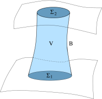
The statement of current conservation $d\star J=0$ means that the electric charge $Q_{e}$ in a region cannot change unless current flows in or out of that region. This fact, familiar from Electromagnetism, also has a nice expression in terms of forms. Consider a cylindrical region of spacetime $V$ , ending on two spatial hypersurfaces $\Sigma_{1}$ and $\Sigma_{2}$ as shown in the figure. The boundary of $V$ is then

\displaystyle\partial V=\Sigma_{1}\cup\Sigma_{2}\cup B

where $B$ is the cylindrical timelike hypersurface.

We require that $J=0$ on $B$ , which is the statement that no current flows in or out of the region. Then we have

\displaystyle Q_{e}(\Sigma_{1})-Q_{e}(\Sigma_{2})=\int_{\Sigma_{1}}\star J-% \int_{\Sigma_{2}}\star J=\int_{\partial V}\star J=\int_{V}d\star J=0

which tells us that the electric charge remains constant in time.

Maxwell Equations Using Connections

The form of the Maxwell equations given above makes no reference to a connection. It does, however, use the metric, buried in the definition of the Hodge $\star$ .

There is an equivalent formulation of the Maxwell equation using the covariant derivative. This will also serve to highlight the relationship between the covariant and exterior derivatives. First note that, given a one-form $A\in\Lambda^{1}(M)$ , we can define the field strength as

\displaystyle F_{\mu\nu}=\nabla_{\mu}A_{\nu}-\nabla_{\nu}A_{\mu}=\partial_{\mu% }A_{\nu}-\partial_{\nu}A_{\mu}

where the Christoffel symbols have cancelled out by virtue of the anti-symmetry. This is what allowed us to define the exterior derivative without the need for a connection.

Next, consider the current one-form $J$ . We can recast the statement of current conservation as follows:

Claim:

\displaystyle d\star J=0\ \ \ \Leftrightarrow\ \ \ \nabla_{\mu}J^{\mu}=0

Proof: We have

\displaystyle\nabla_{\mu}J^{\mu}=\partial_{\mu}J^{\mu}+\Gamma^{\mu}_{\mu\rho}J% ^{\rho}=\frac{1}{\sqrt{-g}}\partial_{\mu}\left(\sqrt{-g}J^{\mu}\right)

where, in the second equality, we have used our previous result (3.113): $\Gamma^{\mu}_{\mu\nu}=\partial_{\nu}\log\sqrt{|g|}$ . But this final form is proportional to $d\star J$ , with the Hodge dual defined in (3.97). $\Box$

As an aside, in Riemannian signature the formula

\displaystyle\nabla_{\mu}J^{\mu}=\frac{1}{\sqrt{g}}\partial_{\mu}(\sqrt{g}J^{% \mu})

provides a quick way of computing the divergence in different coordinate systems (if you don’t have the inside cover of Jackson to hand). For example, in spherical polar coordinates on ${\bf R}^{3}$ , we have $g=r^{4}\sin^{2}\theta$ . Plug this into the expression above to immediately find

\displaystyle\nabla\cdot{\bf J}=\frac{1}{r^{2}}\partial_{r}(r^{2}J^{r})+\frac{% 1}{\sin\theta}\,\partial_{\theta}(\sin\theta\,J^{\theta})+\partial_{\phi}J^{\phi}

The Maxwell equation (3.114) can also be written in terms of the covariant derivative

Claim:

\displaystyle d\star F=\star J\ \ \ \Leftrightarrow\ \ \ \nabla_{\mu}F^{\mu\nu% }=J^{\nu}

(3.116)

Proof: We have

	$\displaystyle\nabla_{\mu}F^{\mu\nu}$	$\displaystyle=$	$\displaystyle\partial_{\mu}F^{\mu\nu}+\Gamma^{\mu}_{\mu\rho}F^{\rho\nu}+\Gamma% ^{\nu}_{\mu\rho}F^{\mu\rho}$
		$\displaystyle=$	$\displaystyle\frac{1}{\sqrt{-g}}\partial_{\mu}\left(\sqrt{-g}F^{\mu\nu}\right)% +\Gamma^{\nu}_{\mu\rho}F^{\mu\rho}=\frac{1}{\sqrt{-g}}\partial_{\mu}\left(% \sqrt{-g}F^{\mu\nu}\right)$

where, in the second equality, we’ve again used (3.113) and in the final equality we’ve used the fact that $\Gamma^{\nu}_{\mu\rho}$ is symmetric while $F^{\mu\rho}$ is anti-symmetric. To complete the proof, you need to chase down the definitions of the Hodge dual (3.97) and the exterior derivative (2.81). (If you’re struggling to match factors of $\sqrt{-g}$ , then remember that the volume form $v=\sqrt{-g}\epsilon$ is a tensor, while the epsilon symbol $\epsilon_{\mu_{1}\ldots\mu_{4}}$ is a tensor density.) $\Box$

3.3 Parallel Transport

Although we have now met a number of properties of the connection, we have not yet explained its name. What does it connect?

The answer is that the connection connects tangent spaces, or more generally any tensor vector space, at different points of the manifold. This map is called parallel transport. As we stressed earlier, such a map is necessary to define differentiation.

Take a vector field $X$ and consider some associated integral curve $C$ , with coordinates $x^{\mu}(\tau)$ , such that

\displaystyle X^{\mu}\Big{|}_{C}=\frac{dx^{\mu}(\tau)}{d\tau}

(3.117)

We say that a tensor field $T$ is parallely transported along $C$ if

\displaystyle\nabla_{X}T=0

(3.118)

Suppose that the curve $C$ connects two points, $p\in M$ and $q\in M$ . The requirement (3.118) provides a map from the vector space defined at $p$ to the vector space defined at $q$ .

To illustrate this, consider the parallel transport of a second vector field $Y$ . In components, the condition (3.118) reads

\displaystyle X^{\nu}\left(\partial_{\nu}Y^{\mu}+\Gamma^{\mu}_{\,\nu\rho}Y^{% \rho}\right)=0

If we now evaluate this on the curve $C$ , we can think of $Y^{\mu}=Y^{\mu}(x(\tau))$ , which obeys

\displaystyle\frac{dY^{\mu}}{d\tau}+X^{\nu}\Gamma^{\mu}_{\,\nu\rho}Y^{\rho}=0

(3.119)

These are a set of coupled, ordinary differential equations. Given an initial condition at, say $\tau=0$ , corresponding to point $p$ , these equations can be solved to find a unique vector at each point along the curve.

Parallel transport is path dependent. It depends on both the connection, and the underlying path which, in this case, is characterised by the vector field $X$ .

This is the second time we’ve used a vector field $X$ to construct maps between tensors at different points in the manifold. In Section 2.2.2, we used $X$ to generate a flow $\sigma_{t}:M\rightarrow M$ , which we could then use to pull-back or push-forward tensors from one point to another. This was the basis of the Lie derivative. This is not the same as the present map. Here, we’re using $X$ only to define the curve, while the connection does the work of relating vector spaces along the curve.

3.3.1 Geodesics Revisited

A geodesic is a curve tangent to a vector field $X$ that obeys

\displaystyle\nabla_{X}X=0

(3.120)

Along the curve $C$ , we can substitute the expression (3.117) into (3.119) to find

\displaystyle\frac{d^{2}x^{\mu}}{d\tau^{2}}+\Gamma^{\mu}{}_{\rho\nu}\frac{dx^{% \rho}}{d\tau}\frac{dx^{\nu}}{d\tau}=0

(3.121)

This is precisely the geodesic equation (1.31) that we derived in Section 1 by considering the action for a particle moving in spacetime. In fact, we find that the condition (3.120) results in geodesics with affine parameterisation.

For the Levi-Civita connection, we have $\nabla_{X}g=0$ . This ensures that for any vector field $Y$ parallely transported along a geodesic $X$ , so $\nabla_{X}Y=\nabla_{X}X=0$ , we have

\displaystyle\frac{d}{d\tau}g(X,Y)=0

This tells us that the vector field $Y$ makes the same angle with the tangent vector along each point of the geodesic.

3.3.2 Normal Coordinates

Geodesics lend themselves to the construction of a particularly useful coordinate system. On a Riemannian manifold, in the neighbourhood of a point $p\in M$ , we can always find coordinates such that

\displaystyle g_{\mu\nu}(p)=\delta_{\mu\nu}\ \ \ {\rm and}\ \ \ g_{\mu\nu,\rho% }(p)=0

(3.122)

The same holds for Lorentzian manifolds, now with $g_{\mu\nu}(p)=\eta_{\mu\nu}$ . These are referred to as normal coordinates. Because the first derivative of the metric vanishes, normal coordinates have the property that, at the point $p$ , the Christoffel symbols vanish: $\Gamma^{\mu}_{\,\nu\rho}(p)=0$ . Generally, away from $p$ we will have $\Gamma^{\mu}_{\,\nu\rho}\neq 0$ . Note, however, that it is not generally possible to ensure that the second derivatives of the metric also vanish. This, in turn, means that it’s not possible to pick coordinates such that the Riemann tensor vanishes at a given point.

There are a number of ways to demonstrate the existence of coordinates (3.122). The brute force way is to start with some metric $\tilde{g}_{\mu\nu}$ in coordinates $\tilde{x}^{\mu}$ and try to find a change of coordinates to $x^{\mu}(\tilde{x})$ which does the trick. In the new coordinates,

\displaystyle\frac{\partial{\tilde{x}^{\rho}}}{\partial{x^{\mu}}}\frac{% \partial{\tilde{x}^{\sigma}}}{\partial{x^{\nu}}}\tilde{g}_{\rho\sigma}=g_{\mu\nu}

(3.123)

We’ll take the point $p$ to be the origin in both sets of coordinates. Then we can Taylor expand

\displaystyle\tilde{x}^{\rho}=\left.\frac{\partial{\tilde{x}^{\rho}}}{\partial% {x^{\mu}}}\right|_{x=0}x^{\mu}+\frac{1}{2}\left.\frac{\partial^{2}\tilde{x}^{% \rho}}{\partial x^{\mu}\partial x^{\nu}}\right|_{x=0}x^{\mu}x^{\nu}+\ldots

We insert this into (3.123), together with a Taylor expansion of $\tilde{g}_{\rho\sigma}$ , and try to solve the resulting partial differential equations to find the coefficients $\partial\tilde{x}/\partial x$ and $\partial^{2}\tilde{x}/\partial x^{2}$ that do the job. For example, the first requirement is

\displaystyle\left.\frac{\partial{\tilde{x}^{\rho}}}{\partial{x^{\mu}}}\right|% _{x=0}\left.\frac{\partial{\tilde{x}^{\sigma}}}{\partial{x^{\nu}}}\right|_{x=0% }\tilde{g}_{\rho\sigma}(p)=\delta_{\mu\nu}

Given any $\tilde{g}_{\rho\sigma}(p)$ , it’s always possible to find $\partial\tilde{x}/\partial x$ so that this is satisfied. In fact, a little counting shows that there are many such choices. If ${\rm dim}M=n$ , then there are $n^{2}$ independent coefficients in the matrix $\partial\tilde{x}/\partial x$ . The equation above puts $\frac{1}{2}n(n+1)$ conditions on these. That still leaves $\frac{1}{2}n(n-1)$ parameters unaccounted for. But this is to be expected: this is precisely the dimension of the rotational group $SO(n)$ (or the Lorentz group $SO(1,n-1)$ ) that leaves the flat metric unchanged.

We can do a similar counting at the next order. There are $\frac{1}{2}n^{2}(n+1)$ independent elements in the coefficients $\partial^{2}\tilde{x}^{\rho}/\partial x^{\mu}\partial x^{\nu}$ . This is exactly the same number of conditions in the requirement $g_{\mu\nu,\rho}(p)=0$ .

We can also see why we shouldn’t expect to set the second derivative of the metric to zero. Requiring $g_{\mu\nu,\rho\sigma}=0$ is $\frac{1}{4}n^{2}(n+1)^{2}$ constraints. Meanwhile, the next term in the Taylor expansion is $\partial^{3}\tilde{x}^{\rho}/\partial x^{\mu}\partial x^{\nu}\partial x^{\lambda}$ which has $\frac{1}{6}n^{2}(n+1)(n+2)$ independent coefficients. We see that the numbers no longer match. This time we fall short, leaving

\displaystyle\frac{1}{4}n^{2}(n+1)^{2}-\frac{1}{6}n^{2}(n+1)(n+2)=\frac{1}{12}% n^{2}(n^{2}-1)

unaccounted for. This, therefore, is the number of ways to characterise the second derivative of the metric in a manner that cannot be undone by coordinate transformations. Indeed, it is not hard to show that this is precisely the number of independent coefficients in the Riemann tensor. (For $n=4$ , there are 20 coefficients of the Riemann tensor.)

Figure 23: Start with a tangent vector, and follow the resulting geodesic to get the exponential map.

The Exponential Map

There is a rather pretty, direct way to construct the coordinates (3.122). This uses geodesics. The rough idea is that, given a tangent vector $X_{p}\in T_{p}(M)$ , there is a unique affinely parameterised geodesic through $p$ with tangent vector $X_{p}$ at $p$ . We then label any point $q$ in the neighbourhood of $p$ by the coordinates of the geodesic that take us to $q$ in some fixed amount of time. It’s like throwing a ball in all possible directions, and labelling points by the initial velocity needed for the ball to reach that point in, say, 1 second.

Let’s put some flesh on this. We introduce any coordinate system (not necessarily normal coordinates) $\tilde{x}^{\mu}$ in the neighbourhood of $p$ . Then the geodesic we want solves the equation (3.121) subject to the requirements

\displaystyle\left.\frac{d\tilde{x}^{\mu}}{d\tau}\right|_{\tau=0}=\tilde{X}^{% \mu}_{p}\ \ \ {\rm with}\ \ \ \tilde{x}^{\mu}(\tau=0)=0

There is a unique solution.

This observation means that we can define a map,

\displaystyle{\rm Exp}:T_{p}(M)\rightarrow M

Given $X_{p}\in T_{p}(M)$ , construct the appropriate geodesic and the follow it for some affine distance which we take to be $\tau=1$ . This gives a point $q\in M$ . This is known as the exponential map and is illustrated in the Figure 23.

There is no reason that the exponential map covers all of the manifold $M$ . It could well be that there are points which cannot be reached from $p$ by geodesics. Moreover, it may be that there are tangent vectors $X_{p}$ for which the exponential map is ill-defined. In general relativity, this occurs if the spacetime has singularities. Neither of these issues are relevant for our current purpose.

Now pick a basis $\{e_{\mu}\}$ of $T_{p}(M)$ . The exponential map means that tangent vector $X_{p}=X^{\mu}e_{\mu}$ defines a point $q$ in the neighbourhood of $p$ . We simply assign this point coordinates

\displaystyle x^{\mu}(q)=X^{\mu}

These are the normal coordinates.

If we pick the initial basis $\{e_{\mu}\}$ to be orthonormal, then the geodesics will point in orthogonal directions which ensures that the metric takes the form $g_{\mu\nu}(p)=\delta_{\mu\nu}$ .

To see that the first derivative of the metric also vanishes, we first fix a point $q$ associated to a given tangent vector $X\in T_{p}(M)$ . This tells us that the point $q$ sits a distance $\tau=1$ along the geodesic. We can now ask: what tangent vector will take us a different distance along this same geodesic? Because the geodesic equation (3.121) is homogeneous in $\tau$ , if we halve the length of $X$ then we will travel only half the distance along the geodesic, i.e. to $\tau=1/2$ . In general, the tangent vector $\tau X$ will take us a distance $\tau$ along the geodesic

\displaystyle{\rm Exp}:\tau X_{p}\rightarrow x^{\mu}(\tau)=\tau X^{\mu}

This means that the geodesics in these coordinates take the particularly simply form

\displaystyle x^{\mu}(\tau)=\tau X^{\mu}

Since these are geodesics, they must solve the geodesic equation (3.121). But, for trajectories that vary linearly in time, this is just

\displaystyle\Gamma^{\mu}_{\,\rho\nu}(x(\tau))\,X^{\rho}X^{\nu}=0

This holds at any point along the geodesic. At most points $x(\tau)$ , this equation only holds for those choices of $X^{\rho}$ which take us along the geodesic in the first place. However, at $x(\tau)=0$ , corresponding to the point $p$ of interest, this equation must hold for any tangent vector $X^{\mu}$ . This means that $\Gamma^{\mu}_{\,(\rho\nu)}(p)=0$ which, for a torsion free connection, ensures that $\Gamma^{\mu}_{\,\rho\nu}(p)=0$ .

Vanishing Christoffel symbols means that the derivative of the metric vanishes. This follows for the Levi-Civita connection by writing $2g_{\mu\sigma}\Gamma^{\sigma}_{\,\rho\nu}=g_{\mu\rho,\nu}+g_{\mu\nu,\rho}-g_{% \rho\nu,\mu}$ . Symmetrising over $(\mu\rho)$ means that the last two terms cancel, leaving us with $g_{\mu\rho,\nu}=0$ when evaluated at $p$ .

The Equivalence Principle

Normal coordinates play an important conceptual role in general relativity. Any observer at point $p$ who parameterises her immediate surroundings using coordinates constructed by geodesics will experience a locally flat metric, in the sense of (3.122).

This is the mathematics underlying the Einstein equivalence principle. This principle states that any freely falling observer, performing local experiments, will not experience a gravitational field. Here “freely falling” means the observer follows geodesics, as we saw in Section 1 and will naturally use normal coordinates. In this context, the coordinates are called a local inertial frame. The lack of gravitational field is the statement that $g_{\mu\nu}(p)=\eta_{\mu\nu}$ .

Key to understanding the meaning and limitations of the equivalence principle is the word “local”. There is a way to distinguish whether there is a gravitational field at $p$ : we compute the Riemann tensor. This depends on the second derivative of the metric and, in general, will be non-vanishing. However, to measure the effects of the Riemann tensor, one typically has to compare the result of an experiment at $p$ with an experiment at a nearby point $q$ : this is considered a “non-local” observation as far as the equivalence principle goes. In the next two subsections, we give examples of physics that depends on the Riemann tensor.

3.3.3 Path Dependence: Curvature and Torsion

Take a tangent vector $Z_{p}\in T_{p}(M)$ , and parallel transport it along a curve $C$ to some point $r\in M$ . Now parallel transport it along a different curve $C^{\prime}$ to the same point $r$ . How do the resulting vectors differ?

To answer this, we construct each of our curves $C$ and $C^{\prime}$ from two segments, generated by linearly independent vector fields, $X$ and $Y$ satisfying $[X,Y]=0$ as shown in Figure 24. To make life easy, we’ll take the point $r$ to be close to the original point $p$ .

We pick normal coordinates $x^{\mu}=(\tau,\sigma,0,\ldots)$ so that the starting point is at $x^{\mu}(p)=0$ while the tangent vectors are aligned along the coordinates, $X=\partial/\partial\tau$ and $Y=\partial/\partial\sigma$ . The other corner points are then $x^{\mu}(q)=(\delta\tau,0,0,\ldots)$ , $x^{\mu}(r)=(\delta\tau,\delta\sigma,0,\ldots)$ and $x^{\mu}(s)=(0,\delta\sigma,0,\ldots)$ where $\delta\tau$ and $\delta\sigma$ are taken to be small. This set-up is shown in Figure 24.

Figure 24: Parallel transporting a vector

Z_{p}

along two different paths does not give the same answer.

First we parallel transport $Z_{p}$ along $X$ to $Z_{q}$ . Along the curve, $Z^{\mu}$ solves (3.119)

\displaystyle\frac{dZ^{\mu}}{d\tau}+X^{\nu}\Gamma^{\mu}_{\,\rho\nu}Z^{\rho}=0

(3.124)

We Taylor expand the solution as

\displaystyle Z^{\mu}_{q}=Z^{\mu}_{p}+\left.\frac{dZ^{\mu}}{d\tau}\right|_{% \tau=0}\delta\tau+\frac{1}{2}\left.\frac{d^{2}Z^{\mu}}{d\tau^{2}}\right|_{\tau% =0}\delta\tau^{2}+{\cal O}(\delta\tau^{3})

From (3.124), we have $dZ^{\mu}/d\tau\big{|}_{0}=0$ because, in normal coordinates, $\Gamma^{\mu}_{\ \rho\nu}(p)=0$ . We can calculate the second derivative by differentiating (3.124) to find

$\displaystyle\left.\frac{d^{2}Z^{\mu}}{d\tau^{2}}\right\|_{\tau=0}$	$\displaystyle=$	$\displaystyle-\left.\left(X^{\nu}Z^{\rho}\frac{d\Gamma^{\mu}_{\,\rho\nu}}{d% \tau}+\frac{dX^{\nu}}{d\tau}Z^{\rho}\Gamma^{\mu}_{\!\rho\nu}+X^{\nu}\frac{dZ^{% \rho}}{d\tau}\Gamma^{\mu}_{\!\rho\nu}\right)\right\|_{p}$
	$\displaystyle=$	$\displaystyle-\left.X^{\nu}Z^{\rho}\frac{d\Gamma^{\mu}_{\,\rho\nu}}{d\tau}% \right\|_{p}$
	$\displaystyle=$	$\displaystyle-(X^{\nu}X^{\sigma}Z^{\rho}\Gamma^{\mu}_{\,\rho\nu,\sigma})_{p}$

Here the second line follows because we’re working in normal coordinates at $p$ , and the final line because $\tau$ is the parameter along the integral curve of $X$ , so $d/d\tau=X^{\sigma}\partial_{\sigma}$ . We therefore have

\displaystyle Z^{\mu}_{q}=Z^{\mu}_{p}-\frac{1}{2}(X^{\nu}X^{\sigma}Z^{\rho}% \Gamma^{\mu}_{\,\rho\nu,\sigma})_{p}\,\delta\tau^{2}+\ldots

(3.126)

Now we parallel transport once more, this time along $Y$ to $Z_{r}^{\mu}$ . The Taylor expansion now takes the form

\displaystyle Z^{\mu}_{r}=Z^{\mu}_{q}+\left.\frac{dZ^{\mu}}{d\sigma}\right|_{q% }\delta\sigma+\frac{1}{2}\left.\frac{d^{2}Z^{\mu}}{d\sigma^{2}}\right|_{q}% \delta\sigma^{2}+{\cal O}(\delta\sigma^{3})

(3.127)

We can again evaluate the first derivative ${dZ^{\mu}}/{d\sigma}|_{q}$ using the analog of the parallel transport equation (3.124),

\displaystyle\left.\frac{dZ^{\mu}}{d\sigma}\right|_{q}=-(Y^{\nu}Z^{\rho}\Gamma% ^{\mu}_{\,\rho\nu})_{q}

Since we’re working in normal coordinates about $p$ and not $q$ , we no longer get to argue that this term vanishes. Instead we Taylor expand about $p$ to get

\displaystyle(Y^{\nu}Z^{\rho}\Gamma^{\mu}_{\,\rho\nu})_{q}=(Y^{\nu}Z^{\rho}X^{% \sigma}\Gamma^{\mu}_{\,\rho\nu,\sigma})_{p}\,\delta\tau+\ldots

Note that in principle we should also Taylor expand $Y^{\nu}$ and $Z^{\rho}$ but, at leading order, these will multiply $\Gamma^{\mu}_{\!\rho\nu}(p)=0$ , so they only contribute at next order. The second order term in the Taylor expansion (3.127) involves $d^{2}Z^{\mu}/d\sigma^{2}|_{q}$ and there is an expression similar to (3.3.3). To leading order the $dX^{\nu}/d\sigma$ and $dZ^{\rho}/d\sigma$ terms are again absent because they are multiplied by $\Gamma^{\mu}_{\,\rho\nu}(q)=d\Gamma^{\mu}_{\,\rho\nu}/d\tau|_{p}\,\delta\tau$ . We therefore have

	$\displaystyle\left.\frac{d^{2}Z^{\mu}}{d\sigma^{2}}\right\|_{q}$	$\displaystyle=$	$\displaystyle-(Y^{\nu}Y^{\sigma}Z^{\rho}\Gamma^{\mu}_{\,\rho\nu,\sigma})_{q}+\ldots$
		$\displaystyle=$	$\displaystyle-(Y^{\nu}Y^{\sigma}Z^{\rho}\Gamma^{\mu}_{\,\rho\nu,\sigma})_{p}+\ldots$

where we replaced the point $q$ with point $p$ because they differ only subleading terms proportional to $\delta\tau$ . The upshot is that this time the difference between $Z_{r}^{\mu}$ and $Z_{q}^{\mu}$ involves two terms,

\displaystyle Z_{r}^{\mu}

\displaystyle=

\displaystyle Z_{q}^{\mu}-(Y^{\nu}Z^{\rho}X^{\sigma}\Gamma^{\mu}_{\,\rho\nu,% \sigma})_{p}\,\delta\tau\delta\sigma-\frac{1}{2}(Y^{\nu}Y^{\sigma}Z^{\rho}% \Gamma^{\mu}_{\,\rho\nu,\sigma})_{p}\,\delta\sigma^{2}+\ldots

Finally, we can relate $Z_{q}^{\mu}$ to $Z_{p}^{\mu}$ using the expression (3.126) that we derived previously. We end up with

\displaystyle Z_{r}^{\mu}

\displaystyle=

\displaystyle Z^{\mu}_{p}-\frac{1}{2}(\Gamma^{\mu}_{\,\rho\nu,\sigma})_{p}% \left[X^{\nu}X^{\sigma}Z^{\rho}\,\delta\tau^{2}+2Y^{\nu}Z^{\rho}X^{\sigma}\,% \delta\sigma\delta\tau+Y^{\nu}Y^{\sigma}Z^{\rho}\,\delta\sigma^{2}\right]_{p}+\ldots

where $\ldots$ denotes any terms cubic or higher in small quantities.

Now suppose we go along the path $C^{\prime}$ , first visiting point $s$ and then making our way to $r$ . We can read the answer off directly from the result above, simply by swapping $X$ and $Y$ and $\sigma$ and $\tau$ ; only the middle term changes,

\displaystyle Z_{r}^{\prime\,\mu}

\displaystyle=

\displaystyle Z^{\mu}_{p}-\frac{1}{2}(\Gamma^{\mu}_{\,\rho\nu,\sigma})_{p}% \left[X^{\nu}X^{\sigma}Z^{\rho}\,\delta\tau^{2}+2X^{\nu}Z^{\rho}Y^{\sigma}\,% \delta\sigma\delta\tau+Y^{\nu}Y^{\sigma}Z^{\rho}\,\delta\sigma^{2}\right]_{p}+\ldots

We find that

	$\displaystyle\Delta Z^{\mu}_{r}=Z^{\mu}_{r}-Z_{r}^{\prime\,\mu}$	$\displaystyle=$	$\displaystyle-(\Gamma^{\mu}_{\,\rho\nu,\sigma}-\Gamma^{\mu}_{\,\rho\sigma,\nu}% )_{p}(Y^{\nu}Z^{\rho}X^{\sigma})_{p}\,\delta\sigma\delta\tau+\ldots$
		$\displaystyle=$	$\displaystyle(R^{\mu}{}_{\rho\sigma\nu}Y^{\nu}Z^{\rho}X^{\sigma})_{p}\,\delta% \sigma\delta\tau+\ldots$

where, in the final equality, we’ve used the expression for the Riemann tensor in components (3.107), which simplifies in normal coordinates as $\Gamma^{\mu}_{\rho\sigma}(p)=0$ . Note that, to the order we’re working, we could equally as well evaluate $R^{\mu}{}_{\rho\sigma\nu}X^{\nu}Z^{\rho}Y^{\sigma}$ at the point $r$ ; the two differ only by higher order terms.

Although our calculation was performed with a particular choice of coordinates, the end result is written as an equality between tensors and must, therefore, hold in any coordinate system. This is a trick that we will use frequently throughout these lectures: calculations are considerably easier in normal coordinates. But if the resulting expression relate tensors then the final result must be true in any coordinate system.

We have discovered a rather nice interpretation of the Riemann tensor: it tells us the path dependence of parallel transport. The calculation above is closely related to the idea of holonomy. Here, one transports a vector around a closed curve $C$ and asks how the resulting vector compares to the original. This too is captured by the Riemann tensor. A particularly simple example of non-trivial holonomy comes from parallel transport of a vector on a sphere: the direction that you end up pointing in depends on the path you take.

The Meaning of Torsion

We discarded torsion almost as soon as we met it, choosing to work with the Levi-Civita connection which has vanishing torsion, $\Gamma^{\rho}_{\,\mu\nu}=\Gamma^{\rho}_{\,\nu\mu}$ . Moreover, as we will see in Section 4, torsion plays no role in the theory of general relativity which makes use of the Levi-Civita connection. Nonetheless, it is natural to ask: what is the geometric meaning of torsion? There is an answer to this that makes use of the kind of parallel transport arguments we used above.

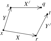
This time, we start with two vectors $X,Y\in T_{p}(M)$ . We pick coordinates $x^{\mu}$ and write these vectors as $X=X^{\mu}\partial_{\mu}$ and $Y=Y^{\mu}\partial_{\mu}$ . Starting from $p\in M$ , we can use these two vectors to construct two points infinitesimally close to $p$ . We call these points $r$ and $s$ respectively: they have coordinates

\displaystyle r:x^{\mu}+X^{\mu}\epsilon\ \ \ {\rm and}\ \ \ s:x^{\mu}+Y^{\mu}\epsilon

where $\epsilon$ is some infinitesimal parameter.

We now parallel transport the vector $X\in T_{p}(M)$ along the direction of $Y$ to give a new vector $X^{\prime}\in T_{s}(M)$ . Similarly, we parallel transport $Y$ along the direction of $X$ to get a new vector $Y^{\prime}\in T_{r}(M)$ . These new vectors have components

\displaystyle X^{\prime}=(X^{\mu}-\epsilon\Gamma^{\mu}_{\,\nu\rho}Y^{\nu}X^{% \rho})\partial_{\mu}\ \ \ {\rm and}\ \ \ Y^{\prime}=(Y^{\mu}-\epsilon\Gamma^{% \mu}_{\,\nu\rho}X^{\nu}Y^{\rho})\partial_{\mu}

Each of these tangent vectors now defines a new point. Starting from point $s$ , and moving in the direction of $X^{\prime}$ , we see that we get a new point $q$ with coordinates

\displaystyle q:x^{\mu}+(X^{\mu}+Y^{\mu})\epsilon-\epsilon^{2}\Gamma^{\mu}_{\,% \nu\rho}Y^{\nu}X^{\rho}

Meanwhile, if we sit at point $r$ and move in the direction of $Y^{\prime}$ , we get to a typically different point, $t$ , with coordinates

\displaystyle t:x^{\mu}+(X^{\mu}+Y^{\mu})\epsilon-\epsilon^{2}\Gamma^{\mu}_{\,% \nu\rho}X^{\nu}Y^{\rho}

We see that if the connection has torsion, so $\Gamma^{\mu}_{\,\nu\rho}\neq\Gamma^{\mu}_{\,\rho\nu}$ , then the two points $q$ and $t$ do not coincide. In other words, torsion measures the failure of the parallelogram shown in figure to close.

3.3.4 Geodesic Deviation

Consider now a one-parameter family of geodesics, with coordinates $x^{\mu}(\tau;s)$ . Here $\tau$ is the affine parameter along the geodesics, all of which are tangent to the vector field $X$ so that, along the surface spanned by $x^{\mu}(\tau,s)$ , we have

\displaystyle X^{\mu}=\left.\frac{\partial{x^{\mu}}}{\partial{\tau}}\right|_{s}

Meanwhile, $s$ labels the different geodesics, as shown in Figure 26. We take the tangent vector in the $s$ direction to be generated by a second vector field $S$ so that,

\displaystyle S^{\mu}=\left.\frac{\partial{x^{\mu}}}{\partial{s}}\right|_{\tau}

The tangent vector $S^{\mu}$ is sometimes called the deviation vector; it takes us from one geodesic to a nearby geodesic with the same affine parameter $\tau$ .

The family of geodesics sweeps out a surface embedded in the manifold. This gives us some freedom in the way we assign coordinates $s$ and $\tau$ . In fact, we can always pick coordinates $s$ and $t$ on the surface such that $S=\partial/\partial s$ and $X=\partial/\partial t$ , ensuring that

\displaystyle[S,X]=0

Roughly speaking, we can do this if we use $\tau$ and $s$ as coordinates on some submanifold of $M$ . Then the vector fields can be written simply as $X=\partial/\partial\tau$ and $S=\partial/\partial s$ and $[X,S]=0$ .

Figure 26: The black lines are geodesics generated by

X

. The red lines label constant

\tau

and are generated by

S

, with

[X,S]=0

We can ask how neighbouring geodesics behave. Do they converge? Or do they move further apart? Now consider a connection $\Gamma$ with vanishing torsion, so that $\nabla_{X}S-\nabla_{S}X=[X,S]$ . Since $[X,S]=0$ , we have

\displaystyle\nabla_{X}\nabla_{X}S=\nabla_{X}\nabla_{S}X=\nabla_{S}\nabla_{X}X% +R(X,S)X

where, in the second equality, we’ve used the expression (3.106) for the Riemann tensor as a differential operator. But $\nabla_{X}X=0$ because $X$ is tangent to geodesics, and we have

\displaystyle\nabla_{X}\nabla_{X}S=R(X,S)X

In index notation, this is

\displaystyle X^{\nu}\nabla_{\nu}(X^{\rho}\nabla_{\rho}S^{\mu})=R^{\mu}{}_{\nu% \rho\sigma}X^{\nu}X^{\rho}S^{\sigma}

If we further restrict to an integral curve $C$ associated to the vector field $X$ , as in (3.117), this equation is sometimes written as

\displaystyle\frac{D^{2}S^{\mu}}{D\tau^{2}}=R^{\mu}{}_{\nu\rho\sigma}X^{\nu}X^% {\rho}S^{\sigma}

(3.128)

where $D/D\tau$ is the covariant derivative along the curve $C$ , defined by $D/D\tau=\frac{\partial{x^{\mu}}}{\partial{\tau}}\nabla_{\mu}$ . The left-hand-side tells us how the deviation vector $S^{\mu}$ changes as we move along the geodesic. In other words, it is the relative acceleration of neighbouring geodesics. We learn that this relative acceleration is controlled by the Riemann tensor.

Experimentally, such geodesic deviations are called tidal forces. We met a simple example in Section 1.2.4.

An Example: the Sphere ${\bf S}^{2}$ Again

It is simple to determine the geodesics on the sphere ${\bf S}^{2}$ of radius $r$ . Using the Christoffel symbols (3.111), the geodesic equations are

\displaystyle\frac{d^{2}\theta}{d\tau^{2}}=\sin\theta\cos\theta\left(\frac{d% \phi}{d\tau}\right)^{2}\ \ \ {\rm and}\ \ \ \frac{d^{2}\phi}{d\tau^{2}}=-2% \frac{\cos\theta}{\sin\theta}\frac{d\phi}{d\tau}\frac{d\theta}{d\tau}

The solutions are great circles. The general solution is a little awkward in these coordinates, but there are two simple solutions.

•

We can set $\theta=\pi/2$ with $\dot{\theta}=0$ and $\dot{\phi}={\rm constant}$ . This is a solution in which the particle moves around the equator. Note that this solution doesn’t work for other values of $\theta$ .
•

We can set $\dot{\phi}=0$ and $\dot{\theta}={\rm constant}$ . These are paths of constant longitude and are geodesics for any constant value of $\phi$ . Note, however, that our coordinates go a little screwy at the poles $\theta=0$ and $\theta=\pi$ .

To illustrate geodesic deviation, we’ll look at the second class of solutions; the particle moves along $\theta=v\tau$ , with the angle $\phi$ specifying the geodesic. This set-up is simple enough that we don’t need to use any fancy Riemann tensor techniques: we can just understand the geodesic deviation using simple geometry. The distance between the geodesic at $\phi=0$ and the geodesic at some other longitude $\phi$ is

\displaystyle s(\tau)=r\phi\sin\theta=r\phi\sin(v\tau)

(3.129)

Now let’s re-derive this result using our fancy technology. The geodesics are generated by the vector field $X^{\theta}=v$ . Meanwhile, the separation between geodesics at a fixed $\tau$ is $S^{\phi}=s(\tau)$ . The geodesic deviation equation in the form (3.128) is

\displaystyle\frac{d^{2}s}{d\tau^{2}}=v^{2}R^{\phi}{}_{\theta\theta\phi}\,s(\tau)

We computed the Riemann tensor for ${\bf S}^{2}$ in (3.112); the relevant component is

\displaystyle R_{\phi\theta\theta\phi}=-r^{2}\sin^{2}\theta\ \ \ \Rightarrow\ % \ \ R^{\phi}{}_{\theta\theta\phi}=g^{\phi\phi}R_{\phi\theta\theta\phi}=-1

(3.130)

and the geodesic deviation equation becomes simply

\displaystyle\frac{d^{2}s}{d\tau^{2}}=-v^{2}s

which is indeed solved by (3.129).

3.4 More on the Riemann Tensor and its Friends

Recall that the components of the Riemann tensor are given by (3.107),

\displaystyle{R^{\sigma}}_{\rho\mu\nu}=\partial_{\mu}\Gamma_{\,\nu\rho}^{% \sigma}-\partial_{\nu}\Gamma_{\,\mu\rho}^{\sigma}+\Gamma_{\,\nu\rho}^{\lambda}% \Gamma_{\,\mu\lambda}^{\sigma}-\Gamma_{\,\mu\rho}^{\lambda}\Gamma_{\,\nu% \lambda}^{\sigma}

(3.131)

We can immediately see that the Riemann tensor is anti-symmetric in the final two indices

\displaystyle{R^{\sigma}}_{\rho\mu\nu}=-{R^{\sigma}}_{\rho\nu\mu}

However, there are also a number of more subtle symmetric properties satisfied by the Riemann tensor when we use the Levi-Civita connection. Logically, we could have discussed this back in Section 3.2. However, it turns out that a number of statements are substantially simpler to prove using normal coordinates introduced in Section 3.3.2.

Claim: If we lower an index on the Riemann tensor, and write $R_{\sigma\rho\mu\nu}=g_{\sigma\lambda}R^{\lambda}{}_{\rho\mu\nu}$ then the resulting object also obeys the following identities

•

$R_{\sigma\rho\mu\nu}=-R_{\sigma\rho\nu\mu}$ .
•

$R_{\sigma\rho\mu\nu}=-R_{\rho\sigma\mu\nu}$ .
•

$R_{\sigma\rho\mu\nu}=R_{\mu\nu\sigma\rho}$ .
•

$R_{\sigma[\rho\mu\nu]}=0$ .

Proof: We work in normal coordinates, with $\Gamma^{\lambda}{}_{\mu\nu}=0$ at a point. The Riemann tensor can then be written as

$\displaystyle R_{\sigma\rho\mu\nu}$	$\displaystyle=$	$\displaystyle g_{\sigma\lambda}\left(\partial_{\mu}\Gamma^{\lambda}{}_{\nu\rho% }-\partial_{\nu}\Gamma^{\lambda}{}_{\mu\rho}\right)$
	$\displaystyle=$	$\displaystyle\frac{1}{2}\left(\partial_{\mu}(\partial_{\nu}g_{\sigma\rho}+% \partial_{\rho}g_{\nu\sigma}-\partial_{\sigma}g_{\nu\rho})-\partial_{\nu}(% \partial_{\mu}g_{\sigma\rho}+\partial_{\rho}g_{\mu\sigma}-\partial_{\sigma}g_{% \mu\rho})\right)$
	$\displaystyle=$	$\displaystyle\frac{1}{2}\left(\partial_{\mu}\partial_{\rho}g_{\nu\sigma}-% \partial_{\mu}\partial_{\sigma}g_{\nu\rho}-\partial_{\nu}\partial_{\rho}g_{\mu% \sigma}+\partial_{\nu}\partial_{\sigma}g_{\mu\rho}\right)$

where, in going to the second line, we used the fact that $\partial_{\mu}g^{\lambda\sigma}=0$ in normal coordinates. The first three symmetries are manifest; the final one follows from a little playing. (It is perhaps quicker to see the final symmetry if we return to the Christoffel symbols where, in normal coordinates, we have $R^{\sigma}{}_{\rho\mu\nu}=\partial_{\mu}\Gamma^{\sigma}{}_{\rho\nu}-\partial_{% \nu}\Gamma^{\sigma}{}_{\rho\mu}$ .) But since the symmetry equations are tensor equations, they must hold in all coordinate systems. $\Box$

Claim: The Riemann tensor also obeys the Bianchi identity

\displaystyle\nabla_{[\lambda}R_{\sigma\rho]\mu\nu}=0

(3.132)

Alternatively, we can anti-symmetrise on the final two indices, in which case this can be written as $R^{\sigma}{}_{\rho[\mu\nu;\lambda]}=0$ .

Proof: We again use normal coordinates, where $\nabla_{\lambda}R_{\sigma\rho\mu\nu}=\partial_{\lambda}R_{\sigma\rho\mu\nu}$ at the point $p$ . Schematically, we have $R=\partial\Gamma+\Gamma\Gamma$ , so $\partial R=\partial^{2}\Gamma+\Gamma\partial\Gamma$ and the final $\Gamma\partial\Gamma$ term is absent in normal coordinates. This means that we just have $\partial R=\partial^{2}\Gamma$ which, in its full coordinated glory, is

\displaystyle\partial_{\lambda}R_{\sigma\rho\mu\nu}=\frac{1}{2}\partial_{% \lambda}\left(\partial_{\mu}\partial_{\rho}g_{\nu\sigma}-\partial_{\mu}% \partial_{\sigma}g_{\nu\rho}-\partial_{\nu}\partial_{\rho}g_{\mu\sigma}+% \partial_{\nu}\partial_{\sigma}g_{\mu\rho}\right)

Now anti-symmetrise on the three appropriate indices to get the result. $\Box$

For completeness, we should mention that the identities $R_{\sigma[\rho\mu\nu]}=0$ and $\nabla_{[\lambda}R_{\sigma\rho]\mu\nu}=0$ (sometimes called the first and second Bianchi identities respectively) are more general, in the sense that they hold for an arbitrary torsion free connection. In contrast, the other two identities, $R_{\sigma\rho\mu\nu}=-R_{\rho\sigma\mu\nu}$ and $R_{\sigma\rho\mu\nu}=R_{\mu\nu\sigma\rho}$ hold only for the Levi-Civita connection.

3.4.1 The Ricci and Einstein Tensors

There are a number of further tensors that we can build from the Riemann tensor.

First, given a rank $(1,3)$ tensor, we can always construct a rank $(0,2)$ tensor by contraction. If we start with the Riemann tensor, the resulting object is called the Ricci tensor. It is defined by

\displaystyle R_{\mu\nu}={R^{\rho}}_{\mu\rho\nu}

The Ricci tensor inherits its symmetry from the Riemann tensor. We write $R_{\mu\nu}=g^{\sigma\rho}R_{\sigma\mu\rho\nu}=g^{\rho\sigma}R_{\rho\nu\sigma\mu}$ , giving us

\displaystyle R_{\mu\nu}=R_{\nu\mu}

We can go one step further and create a function $R$ over the manifold. This is the Ricci scalar,

\displaystyle R=g^{\mu\nu}R_{\mu\nu}

The Bianchi identity (3.132) has a nice implication for the Ricci tensor. If we write the Bianchi identity out in full, we have

			$\displaystyle\nabla_{\lambda}R_{\sigma\rho\mu\nu}+\nabla_{\sigma}R_{\rho% \lambda\mu\nu}+\nabla_{\rho}R_{\lambda\sigma\mu\nu}=0$
	$\displaystyle\times\ g^{\mu\lambda}g^{\rho\nu}\ \ \ \Rightarrow$		$\displaystyle\nabla^{\mu}R_{\mu\sigma}-\nabla_{\sigma}R+\nabla^{\nu}R_{\nu% \sigma}=0$

which means that

\displaystyle\nabla^{\mu}R_{\mu\nu}=\frac{1}{2}\nabla_{\nu}R

This motivates us to introduce the Einstein tensor,

\displaystyle G_{\mu\nu}=R_{\mu\nu}-\frac{1}{2}Rg_{\mu\nu}

which has the property that it is covariantly constant, meaning

\displaystyle\nabla^{\mu}G_{\mu\nu}=0

(3.133)

We’ll be seeing much more of the Ricci and Einstein tensors in the next section.

3.4.2 Connection 1-forms and Curvature 2-forms

Calculating the components of the Riemann tensor is straightforward but extremely tedious. It turns out that there is a slightly different way of repackaging the connection and the torsion and curvature tensors using the language of forms. This not only provides a simple way to actually compute the Riemann tensor, but also offers some useful conceptual insight.

Vielbeins

Until now, we have typically worked with a coordinate basis $\{e_{\mu}\}=\{\partial_{\mu}\}$ . However, we could always pick a basis of vector fields that has no such interpretation. For example, a linear combination of a coordinate basis, say

\displaystyle\hat{e}_{a}={e_{a}}^{\mu}\,\partial_{\mu}

will not, in general, be a coordinate basis itself.

Given a metric, there is a non-coordinate basis that will prove particularly useful for computing the curvature tensor. This is the basis such that, on a Riemannian manifold,

\displaystyle g(\hat{e}_{a},\hat{e}_{b})=g_{\mu\nu}{e_{a}}^{\mu}{e_{b}}^{\nu}=% \delta_{ab}

Alternatively, on a Lorentzian manifold we take

\displaystyle g(\hat{e}_{a},\hat{e}_{b})=g_{\mu\nu}{e_{a}}^{\mu}{e_{b}}^{\nu}=% \eta_{ab}

(3.134)

The components ${e_{a}}^{\mu}$ are called vielbeins or tetrads. (On an $n$ -dimensional manifold, these objects are usually called “German word for $n$ ”-beins. For example, one-dimensional manifolds have einbeins; four-dimensional manifolds have vierbeins.)

The is reminiscent of our discussion in Section 3.1.2 where we mentioned that we can always find coordinates so that any metric will look flat at a point. In (3.134), we’ve succeeded in making the manifold look flat everywhere (at least in a patch covered by a chart). There are no coordinates that do this, but there’s nothing to stop us picking a basis of vector fields that does the job. In what follows, $\mu\nu$ indices are raised/lowered with the metric $g_{\mu\nu}$ while $a, b$ indices are raised/lowered with the flat metric $\delta_{ab}$ or $\eta_{ab}$ . We will phrase our discussion in the context of Lorentzian manifolds, with an eye to later applications to general relativity.

The vielbeins aren’t unique. Given a set of vielbeins, we can always find another set related by

\displaystyle\tilde{e}_{a}{}^{\mu}={e_{b}}^{\mu}(\Lambda^{-1})^{b}_{\ a}\ \ \ % {\rm with}\ \ \ \Lambda_{a}^{\ c}\Lambda_{b}^{\ d}\eta_{cd}=\eta_{ab}

(3.135)

These are Lorentz transformations. However now they are local Lorentz transformation, because $\Lambda$ can vary over the manifold. These local Lorentz transformations are a redundancy in the definition of the vielbeins in (3.134).

The dual basis of one-forms $\{\hat{\theta}^{a}\}$ is defined by $\hat{\theta}^{a}(\hat{e}_{b})=\delta^{a}_{b}$ . They are related to the coordinate basis by

\displaystyle\hat{\theta}^{a}={e^{a}}_{\mu}dx^{\mu}

Note the different placement of indices: ${e^{a}}_{\mu}$ is the inverse of ${e_{a}}^{\mu}$ , meaning it satisfies ${e^{a}}_{\mu}{e_{b}}^{\mu}=\delta^{a}_{b}$ and ${e^{a}}_{\mu}{e_{a}}^{\nu}=\delta^{\nu}_{\mu}$ . In the non-coordinate basis, the metric on a Lorentzian manifold takes the form

\displaystyle g=g_{\mu\nu}dx^{\mu}\otimes dx^{\nu}=\eta_{ab}\hat{\theta}^{a}% \otimes\hat{\theta}^{b}\ \ \ \Rightarrow\ \ \ g_{\mu\nu}={e^{a}}_{\mu}{e^{b}}_% {\nu}\eta_{ab}

For Riemannian manifolds, we replace $\eta_{ab}$ with $\delta_{ab}$ .

The Connection One-Form

Given a non-coordinate basis $\{\hat{e}_{a}\}$ , we can define the components of a connection in the usual way (3.100)

\displaystyle\nabla_{\hat{e}_{c}}\hat{e}_{b}=\Gamma^{a}_{cb}\,\hat{e}_{a}

Note that, annoyingly, these are not the same functions as $\Gamma^{\mu}_{\!\rho\nu}$ , which are the components of the connection computed in the coordinate basis! You need to pay attention to whether the components are Greek $\mu,\nu$ etc which tells you that we’re in the coordinate basis, or Roman $a, b$ etc which tells you we’re in the vielbein basis.

We then define the matrix-valued connection one-form as

\displaystyle{\omega^{a}}_{b}=\Gamma^{a}_{cb}\,\hat{\theta}^{c}

(3.136)

This is sometimes referred to as the spin connection because of the role it plays in defining spinors on curved spacetime. We’ll describe this in Section 4.5.6.

The connection one-forms don’t transform covariantly under local Lorentz transformations (3.135). Instead, in the new basis, the components of the connection one-form are defined as $\nabla_{\hat{\,\tilde{e}}_{b}}\hat{\,\tilde{e}}_{c}=\tilde{\Gamma}^{a}_{bc}% \hat{\tilde{e}}_{a}$ . You can check that the connection one-form transforms as

\displaystyle\tilde{\omega}^{a}_{\ b}=\Lambda^{a}_{\ c}\,\omega^{c}_{\ d}(% \Lambda^{-1})^{d}_{\ b}+\Lambda^{a}_{\ c}(d\Lambda^{-1})^{c}_{\ b}

(3.137)

The second term reflects the fact that the original connection components $\Gamma^{\mu}_{\nu\rho}$ do not transform as a tensor, but with an extra term involving the derivative of the coordinate transformation (3.105). This now shows up as an extra term involving the derivative of the local Lorentz transformation.

There is a rather simple way to compute the connection one-forms, at least for a torsion free connection. This follows from the first of two Cartan structure relations:

Claim: For a torsion free connection,

\displaystyle d\hat{\theta}^{a}+{\omega^{a}}_{b}\wedge\hat{\theta}^{b}=0

(3.138)

Proof: We first look at the second term,

\displaystyle{\omega^{a}}_{b}\wedge\hat{\theta}^{b}=\Gamma^{a}_{cb}\,(e^{c}_{% \ \mu}dx^{\mu})\wedge(e^{b}_{\ \nu}dx^{\nu})

The components $\Gamma^{a}_{\ cb}$ are related to the coordinate basis components by

\displaystyle\Gamma^{a}_{cb}=e^{a}{}_{\rho}e_{c}^{\ \mu}\left(\partial_{\mu}e_% {b}^{\ \rho}+e_{b}^{\ \nu}\Gamma_{\mu\nu}^{\rho}\right)=e^{a}{}_{\rho}e_{c}{}^% {\mu}\nabla_{\mu}e_{b}{}^{\rho}

(3.139)

	$\displaystyle{\omega^{a}}_{b}\wedge\hat{\theta}^{b}$	$\displaystyle=$	$\displaystyle e^{a}{}_{\rho}e_{c}^{\ \lambda}e^{c}_{\ \mu}e^{b}_{\ \nu}\left(% \partial_{\lambda}e_{b}^{\ \rho}+e_{b}^{\ \sigma}\Gamma_{\lambda\sigma}^{\rho}% \right)dx^{\mu}\wedge dx^{\nu}$
		$\displaystyle=$	$\displaystyle e^{a}{}_{\rho}e^{b}_{\ \nu}\partial_{\mu}e_{b}^{\ \rho}\,dx^{\mu% }\wedge dx^{\nu}$

where, in the second line we’ve used $e_{c}{}^{\lambda}e^{c}{}_{\mu}=\delta^{\lambda}_{\mu}$ and the fact that the connection is torsion free so $\Gamma_{[\mu\nu]}^{\rho}=0$ . Now we use the fact that $e^{b}{}_{\nu}e_{b}{}^{\rho}=\delta_{\nu}^{\rho}$ , so $e^{b}{}_{\nu}\partial_{\mu}e_{b}{}^{\rho}=-e_{b}{}^{\rho}\partial_{\mu}e^{b}{}% _{\nu}$ . We have

	$\displaystyle{\omega^{a}}_{b}\wedge\hat{\theta}^{b}$	$\displaystyle=$	$\displaystyle-e^{a}{}_{\rho}e_{b}^{\ \rho}\partial_{\mu}e^{b}_{\ \nu}\,dx^{\mu% }\wedge dx^{\nu}$
		$\displaystyle=$	$\displaystyle-\partial_{\mu}e^{a}{}_{\nu}\,dx^{\mu}\wedge dx^{\nu}=-d\hat{% \theta}^{a}$

which completes the proof. $\Box$

The discussion above was for a general connection. For the Levi-Civita connection, we have a stronger result

Claim: For the Levi-Civita connection, the connection one-form is anti-symmetric

\displaystyle\omega_{ab}=-\omega_{ba}

(3.140)

Proof: This follows from the explicit expression (3.139) for the components $\Gamma^{a}_{bc}$ . Lowering an index, we have

\displaystyle\Gamma_{abc}=\eta_{ad}\,e^{d}{}_{\rho}e_{b}{}^{\mu}\nabla_{\mu}e_% {c}{}^{\rho}=-\eta_{ad}\,e_{c}{}^{\rho}e_{b}{}^{\mu}\nabla_{\mu}e^{d}{}_{\rho}% =-\eta_{cf}e^{f}{}_{\sigma}e_{b}{}^{\mu}\nabla_{\mu}(\eta_{ad}g^{\rho\sigma}e^% {d}{}_{\rho})

where, in the final equality, we’ve used the fact that the connection is compatible with the metric to raise the indices of $e^{d}{}_{\rho}$ inside the covariant derivative. Finishing off the derivation, we then have

\displaystyle\Gamma_{abc}=-\eta_{cf}\,e^{f}{}_{\rho}e_{b}{}^{\mu}\nabla_{\mu}e% _{a}{}^{\rho}=-\Gamma_{cba}

The result then follows from the definition $\omega_{ab}=\Gamma_{acb}\hat{\theta}^{c}$ . $\Box$

The Cartan structure equation (3.138), together with the anti-symmetry condition (3.140), gives a quick way to compute the spin connection. It’s instructive to do some counting to see how these two equations uniquely define $\omega^{a}{}_{b}$ . In particular, since $\omega_{ab}$ is anti-symmetric, one might think that it has $\frac{1}{2}n(n-1)$ independent components, and these can’t possibly be fixed by the $n$ Cartan structure equations (3.138). But this is missing the fact that $\omega_{ab}$ are not numbers, but are one-forms. So the true number of components in $\omega_{ab}$ is $n\times\frac{1}{2}n(n-1)$ . Furthermore, the Cartan structure equation is an equation relating 2-forms, each of which has $\frac{1}{2}n(n-1)$ components. This means that it’s really $n\times\frac{1}{2}n(n-1)$ equations. We see that the counting does work, and the two fix the spin connection uniquely.

The Curvature Two-Form

We can compute the components of the Riemann tensor in our non-coordinate basis,

\displaystyle{R^{a}}_{bcd}=R(\hat{\theta}^{a};\hat{e}_{c},\hat{e}_{d},\hat{e}_% {b})

The anti-symmetry of the last two indices, ${R^{a}}_{bcd}=-{R^{a}}_{bdc}$ , makes this ripe for turning into a matrix of two-forms,

\displaystyle{\cal R}^{a}{}_{b}=\frac{1}{2}R^{a}{}_{bcd}\,\hat{\theta}^{c}% \wedge\hat{\theta}^{d}

(3.141)

The second of the two Cartan structure relations states that this can be written in terms of the curvature one-form as

\displaystyle{\cal R}^{a}{}_{b}=d\omega^{a}{}_{b}+\omega^{a}{}_{c}\wedge\omega% ^{c}{}_{b}

(3.142)

The proof of this is mechanical and somewhat tedious. It’s helpful to define the quantities $[\hat{e}_{a},\hat{e}_{b}]=f_{ab}{}^{c}\,\hat{e}_{c}$ along the way, since they appear on both left and right-hand sides.

3.4.3 An Example: the Schwarzschild Metric

The connection one-form and curvature two-form provide a slick way to compute the curvature tensor associated to a metric. The reason for this is that computing exterior derivatives takes significantly less effort than computing covariant derivatives. We will illustrate this for metrics of the form,

\displaystyle ds^{2}=-f(r)^{2}dt^{2}+f(r)^{-2}dr^{2}+r^{2}(d\theta^{2}+\sin^{2% }\theta\,d\phi^{2})

(3.143)

For later applications, it will prove useful to compute the Riemann tensor for this metric with general $f(r)$ . However, if we want to restrict to the Schwarzschild metric we can take

\displaystyle f(r)=\sqrt{1-\frac{2GM}{r}}

(3.144)

The basis of non-coordinate one-forms is

\displaystyle\hat{\theta}^{0}=f\,dt\ \ ,\ \ \hat{\theta}^{1}=f^{-1}\,dr\ \ ,\ % \ \hat{\theta}^{2}=r\,d\theta\ \ ,\ \ \hat{\theta}^{3}=r\sin\theta\,d\phi

(3.145)

Note that the one-forms $\hat{\theta}$ should not be confused with the angular coordinate $\theta$ ! In this basis, the metric takes the simple form

\displaystyle ds^{2}=\eta_{ab}\hat{\theta}^{a}\otimes\hat{\theta}^{b}

We now compute $d\hat{\theta}^{a}$ . Calculationally, this is straightforward. In particular, it’s substantially easier than computing the covariant derivative because there’s no messy connection to worry about. The exterior derivatives are simply

\displaystyle d\hat{\theta}^{0}=f^{\prime}\,dr\wedge dt\ \ ,\ \ d\hat{\theta}^% {1}=0\ \ ,\ \ d\hat{\theta}^{2}=dr\wedge d\theta\ \ ,\ \ d\hat{\theta}^{3}=% \sin\theta\,dr\wedge d\phi+r\cos\theta\,d\theta\wedge d\phi

The first Cartan structure relation, $d\hat{\theta}^{a}=-\omega^{a}{}_{b}\wedge\hat{\theta}^{b}$ , can then be used to read off the connection one-form. The first equation tells us that $\omega^{0}{}_{1}=f^{\prime}fdt=f^{\prime}\,\hat{\theta}^{0}$ . We then use the anti-symmetry (3.140), together with raising and lowering by the Minkowski metric $\eta={\rm diag}(-1,+1,+1,+1)$ to get $\omega^{1}{}_{0}=\omega_{10}=-\omega_{01}=\omega^{0}{}_{1}$ . The Cartan structure equation then gives $d\hat{\theta}^{1}=-\omega^{1}{}_{0}\wedge\hat{\theta}^{0}+\ldots$ and the $\omega^{1}{}_{0}\wedge\hat{\theta}^{0}$ contribution happily vanishes because it is proportional to $\hat{\theta}^{0}\wedge\hat{\theta}^{0}=0$ .

Next, we take $\omega^{2}{}_{1}=fd\theta=(f/r)\hat{\theta}^{2}$ to solve the $d\hat{\theta}^{2}$ structure equation. The anti-symmetry (3.140) gives $\omega^{1}{}_{2}=-\omega^{2}{}_{1}=-(f/r)\hat{\theta}^{2}$ and this again gives a vanishing contribution to the $d\hat{\theta}^{1}$ structure equation.

Finally, the $d\hat{\theta}^{3}$ equation suggests that we take $\omega^{3}{}_{1}=f\sin\theta d\phi=(f/r)\hat{\theta}^{3}$ and $\omega^{3}{}_{2}=\cos\theta d\phi=(1/r)\cot\theta\,\hat{\theta}^{3}$ . These anti-symmetric partners $\omega^{1}{}_{3}=-\omega^{3}{}_{1}$ and $\omega^{2}{}_{3}=-\omega^{3}{}_{2}$ do nothing to spoil the $d\hat{\theta}^{1}$ and $d\hat{\theta}^{2}$ structure equations, so we’re home dry. The final result is

	$\displaystyle\omega^{0}{}_{1}=\omega^{1}{}_{0}=f^{\prime}\,\hat{\theta}^{0}$	$\displaystyle,$	$\displaystyle\ \ \omega^{2}{}_{1}=-\omega^{1}{}_{2}=\frac{f}{r}\hat{\theta}^{2}$
	$\displaystyle\omega^{3}{}_{1}=-\omega^{1}{}_{3}=\frac{f}{r}\hat{\theta}^{3}$	$\displaystyle,$	$\displaystyle\ \ \omega^{3}{}_{2}=-\omega^{2}{}_{3}=\frac{\cot\theta}{r}\hat{% \theta}^{3}$

Now we can use this to compute the curvature two-form. We will focus on

\displaystyle{\cal R}^{0}{}_{1}=d\omega^{0}{}_{1}+\omega^{0}{}_{c}\wedge\omega% ^{c}{}_{1}

We have

\displaystyle d\omega^{0}{}_{1}=f^{\prime}d\hat{\theta}^{0}+f^{\prime\prime}dr% \wedge\hat{\theta}^{0}=\Big{(}(f^{\prime})^{2}+f^{\prime\prime}f\Big{)}dr% \wedge dt

The second term in the curvature 2-form is $\omega^{0}{}_{c}\wedge\omega^{c}{}_{1}=\omega^{0}{}_{1}\wedge\omega^{1}{}_{1}=0$ . So we’re left with

\displaystyle{\cal R}^{0}{}_{1}=\Big{(}(f^{\prime})^{2}+f^{\prime\prime}f\Big{% )}dr\wedge dt=\Big{(}(f^{\prime})^{2}+f^{\prime\prime}f\Big{)}\hat{\theta}^{1}% \wedge\hat{\theta}^{0}

The other curvature 2-forms can be computed in a similar fashion. We can now read off the components of the Riemann tensor in the non-coordinate basis using (3.141). (We should remember that we get a contribution from both $R^{0}_{\ 101}$ and $R^{0}_{\ 110}=-R^{0}_{\ 101}$ , which cancels the factor of $1/2$ in (3.141).) After lowering an index, we find that the non-vanishing components of the Riemann tensor are

$\displaystyle R_{0101}$	$\displaystyle=$	$\displaystyle ff^{\prime\prime}+(f^{\prime})^{2}$
$\displaystyle R_{0202}$	$\displaystyle=$	$\displaystyle\frac{ff^{\prime}}{r}$
$\displaystyle R_{0303}$	$\displaystyle=$	$\displaystyle\frac{ff^{\prime}}{r}$
$\displaystyle R_{1212}$	$\displaystyle=$	$\displaystyle-\frac{ff^{\prime}}{r}$
$\displaystyle R_{1313}$	$\displaystyle=$	$\displaystyle-\frac{ff^{\prime}}{r}$
$\displaystyle R_{2323}$	$\displaystyle=$	$\displaystyle\frac{1-f^{2}}{r^{2}}$

We can also convert this back to the coordinates $x^{\mu}=(t,r,\theta,\phi)$ using

\displaystyle R_{\mu\nu\rho\sigma}=e^{a}_{\ \mu}e^{b}_{\ \nu}e^{c}_{\ \rho}e^{% d}_{\ \sigma}R_{abcd}

This is particularly easy in this case because the matrices $e_{a}^{\ \mu}$ defining the one-forms (3.145) are diagonal. We then have

$\displaystyle R_{trtr}$	$\displaystyle=$	$\displaystyle ff^{\prime\prime}+(f^{\prime})^{2}$
$\displaystyle R_{t\theta t\theta}$	$\displaystyle=$	$\displaystyle f^{3}f^{\prime}r$
$\displaystyle R_{t\phi t\phi}$	$\displaystyle=$	$\displaystyle f^{3}f^{\prime}r\sin^{2}\theta$
$\displaystyle R_{r\theta r\theta}$	$\displaystyle=$	$\displaystyle-\frac{f^{\prime}r}{f}$	(3.146)
$\displaystyle R_{r\phi r\phi}$	$\displaystyle=$	$\displaystyle-\frac{f^{\prime}r}{f}\sin^{2}\theta$
$\displaystyle R_{\theta\phi\theta\phi}$	$\displaystyle=$	$\displaystyle(1-f^{2})r^{2}\sin^{2}\theta$

Finally, if we want to specialise to the Schwarzschild metric with $f(r)$ given by (3.144), we have

$\displaystyle R_{trtr}$	$\displaystyle=$	$\displaystyle-\frac{2GM}{r^{3}}$
$\displaystyle R_{t\theta t\theta}$	$\displaystyle=$	$\displaystyle\frac{GM(r-2GM)}{r^{2}}$
$\displaystyle R_{t\phi t\phi}$	$\displaystyle=$	$\displaystyle\frac{GM(r-2GM)}{r^{2}}\sin^{2}\theta$
$\displaystyle R_{r\theta r\theta}$	$\displaystyle=$	$\displaystyle-\frac{GM}{r-2GM}$
$\displaystyle R_{r\phi r\phi}$	$\displaystyle=$	$\displaystyle-\frac{GM\sin^{2}\theta}{r-2GM}$
$\displaystyle R_{\theta\phi\theta\phi}$	$\displaystyle=$	$\displaystyle 2GMr\sin^{2}\theta$

Although the calculation is a little lengthy, it turns out to be considerably quicker than first computing the Levi-Civita connection and subsequently motoring through to get the Riemann tensor components.

3.4.4 The Relation to Yang-Mills Theory

It is no secret that the force of gravity is geometrical. However, the other forces are equally as geometrical. The underlying geometry is something called a fibre bundle, rather than the geometry of spacetime.

We won’t describe fibre bundles in this course, but we can exhibit a clear similarity between the structures that arise in general relativity and the structures that arise in the other forces, which are described by Maxwell theory and its generalisation to Yang-Mills theory.

Yang-Mills theory is based on a Lie group $G$ which, for this discussion, we will take to be $SU(N)$ or $U(N)$ . If we take $G=U(1)$ , then Yang-Mills theory reduces to Maxwell theory. The theory is described in terms of an object that physicists call a gauge potential. This is a spacetime “vector” $A_{\mu}$ which lives in the Lie algebra of $G$ . In more down to earth terms, each component is an anti-Hermitian $N\times N$ matrix, $(A_{\mu})^{a}_{\ b}$ , with $a,b=1,\ldots,N$ . In fact, as we saw above, this “vector” is really a one-form. The novelty is that it’s a Lie algebra-valued one-form.

Mathematicians don’t refer to $A_{\mu}$ as a gauge potential. Instead, they call it a connection (on a fibre bundle). This relationship becomes clearer if we look at how $A_{\mu}$ changes under a gauge transformation

\displaystyle\tilde{A}_{\mu}=\Omega A_{\mu}\Omega^{-1}+\Omega\partial_{\mu}% \Omega^{-1}

where $\Omega(x)\in G$ . This is identical to the transformation property (3.137) of the one-form connection under local Lorentz transformations.

In Yang-Mills, as in Maxwell theory, we construct a field strength. In components, this is given by

\displaystyle(F_{\mu\nu})^{a}_{\ b}=\partial_{\mu}(A_{\nu})^{a}_{\ b}-\partial% _{\nu}(A_{\mu})^{a}_{\ b}+[A_{\mu},A_{\nu}]^{a}_{\ b}

Alternatively, in the language of forms, the field strength becomes

\displaystyle F^{a}_{\ b}=dA^{a}{}_{b}+A^{a}{}_{c}\wedge A^{c}{}_{b}

Again, there is an obvious similarity with the curvature 2-form introduced in (3.142). Mathematicians refer to the Yang-Mills field strength the “curvature”.

A particularly quick way to construct the Yang-Mills field strength is to take the commutator of two covariant derivatives. It is simple to check that

\displaystyle[{\cal D}_{\mu},{\cal D}_{\nu}]=F_{\mu\nu}

where I’ve suppressed the $a, b$ indices on both sides. This is the gauge theory version of the Ricci identity (3.108): for a torsion free connection,

\displaystyle[\nabla_{\mu},\nabla_{\nu}]Z^{\sigma}={R^{\sigma}}_{\rho\mu\nu}Z^% {\rho}