Solving the Wave Equation and Diffusion Equation in 2 dimensions
We have seen in other places how to use finite differences to solve PDEs. For example in 1 dimension. Expanding these methods to 2 dimensions does not require significantly more work.
Contents
The Theory
Much like the theory for 1 dimension, we discretize our partial differential equation in space and time and solve the resulting system. How we discretize might depend on the choice of semi-discretization but the principle is similar.
Similarly for 1 dimension we want to investigate the stability of the methods employed. Again, the methods described for 1d work just as well for 2d as discussed in Lecture 9
Implementation
The key problem to overcome when implementing any of the methods involved in this demonstration is generating the matrix form of the Laplacian. However, MATLAB® has some functions which are suited to this problem.
function A = laplacian ( n )
I = speye(n,n);
E = sparse(2:n,1:n-1,1,n,n);
D = E+E'-2*I;
A = kron(D,I)+kron(I,D);
This function returns the matrix Laplacian for a grid of size  using the natural ordering. In fact this code comes from the MATLAB® documentation for kron
The GUI
pde_gui
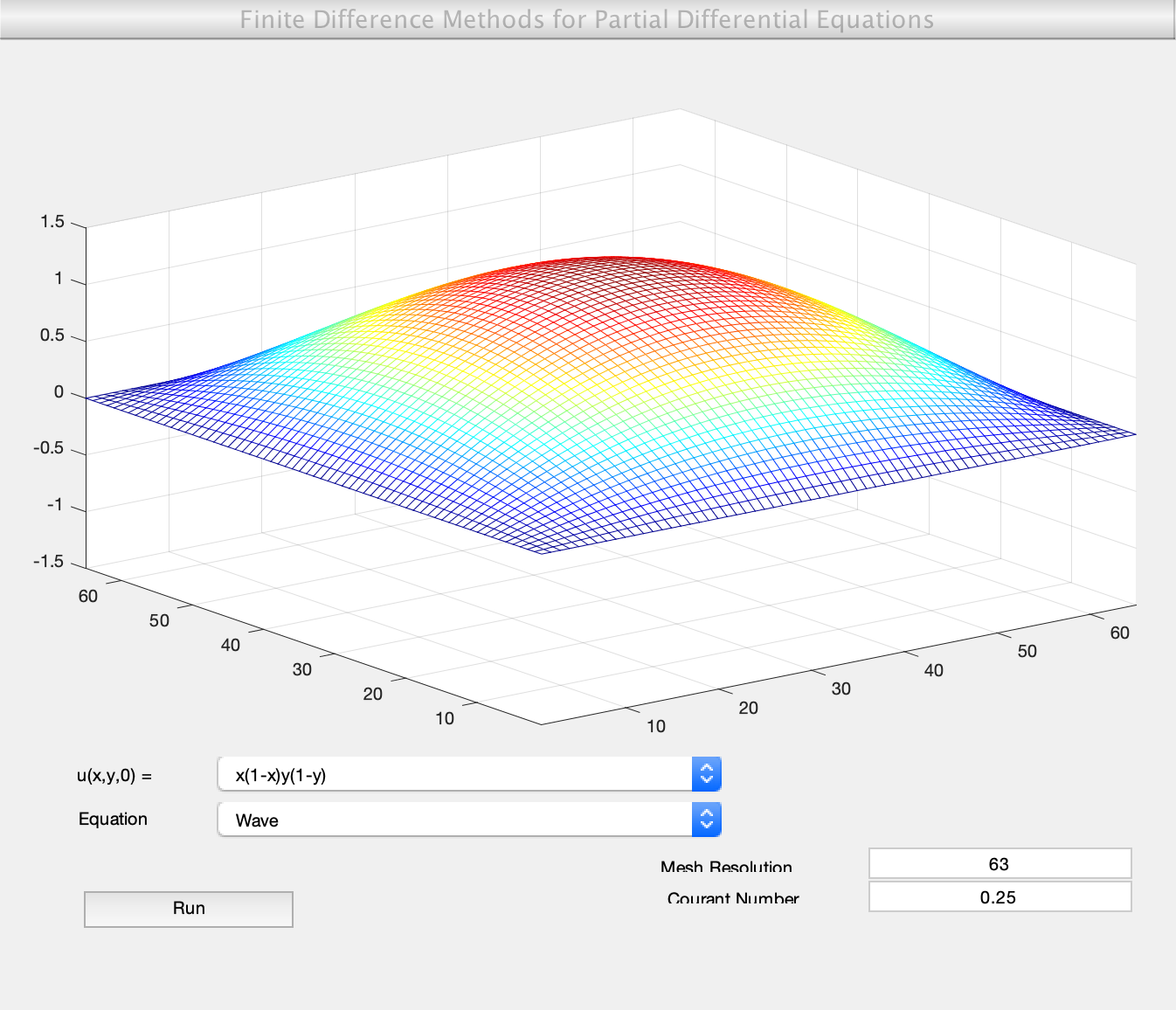
It is possible to choose from three different methods for solving two different PDEs (Wave Equation and Diffusion Equation). There are several different options for grid size and Courant number.
Code
- pde_gui.m (Run this)
- pde_gui.fig (Required - GUI figure)
All files as .zip archive: pdes_2d_all.zip