Fourier Transforms and Fast Fourier Transforms

Spectral convergence, the fast Fourier transform and Fourier theory are all reasons why the Discrete Fourier Transform is so important to Numerical Analysts. It is important to appreciate they all relate to each other:

Contents

Discrete Fourier Transform as an approximation to the Fourier Transform

First we will set up some notation for Fourier Transforms and Discrete Fourier transforms

$\hat{f}_k = \frac{1}{2} \int_{-1}^{1} f(\tau) e^{-i \pi k \tau} \, d\tau, k \in \mathbf{Z}$

$X_{k} = \sum_{n=0}^{N-1} f(\frac{n+1-\frac{N}{2}}{N/2}) e^{-2 \pi i k n/N}\, k = 0, \ldots N-1$

As in the notes, we then approximate:

$\hat{f}_k = \frac{1}{2} \int_{-1}^{1} f(\tau) e^{-i \pi k \tau} \, d\tau$

$\approx \frac{1}{2} \frac{2}{N} \sum_{k = -N/2+1}^{N/2} f(\frac{2k}{N}) e^{- i \pi n \frac{2 k}{N}}$

$= \frac{1}{N} \sum_{k = 0}^{N-1} f( \frac{2(k-N/2+1)}{N}) e^{-i \pi n \left ( \frac{2(k-N/2+1)}{N} \right ) }$

$= \left ( \frac{1}{N} \sum_{k = 0}^{N-1} f( \frac{2(k-N/2+1)}{N}) e^{ \frac{-2 \pi i n k}{N}} \right ) e^{ 2 \pi i n ( \frac{1}{2} + \frac{1}{N} )}$

$= X_k e^{ 2 \pi i n ( \frac{1}{2} + \frac{1}{N})}$

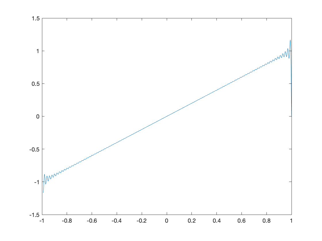
How good is this approximation? Well, we prove in the notes that it converges spectrally so it is a very good approximation. However, the finite truncation does illustrate some strange behaviour. For instance, consider $f(x) = x, x \in [-1,1]$.

N = 200;
x = linspace(-1+2/N,1,N);
f = @(x)(x.^1);

c = exp(2*pi*1i*(N/2 + 1) * [0:N/2 (-N/2+1):-1] /N);
X = 1/N *fft(f(x)); % Compute the DFT
fourier = 0.5*quadv(@(x)(f(x) .* exp(-pi*1i*x* [0:N/2 (-N/2+1):-1])),-1,1); % Compute the actual fourier coefficients

y = linspace(-1 + 2/N,1,1000);
figure(1);
plot(y,real(fourier_val(fourier,y))); % Plot the truncated fourier series
drawnow;

figure(2);
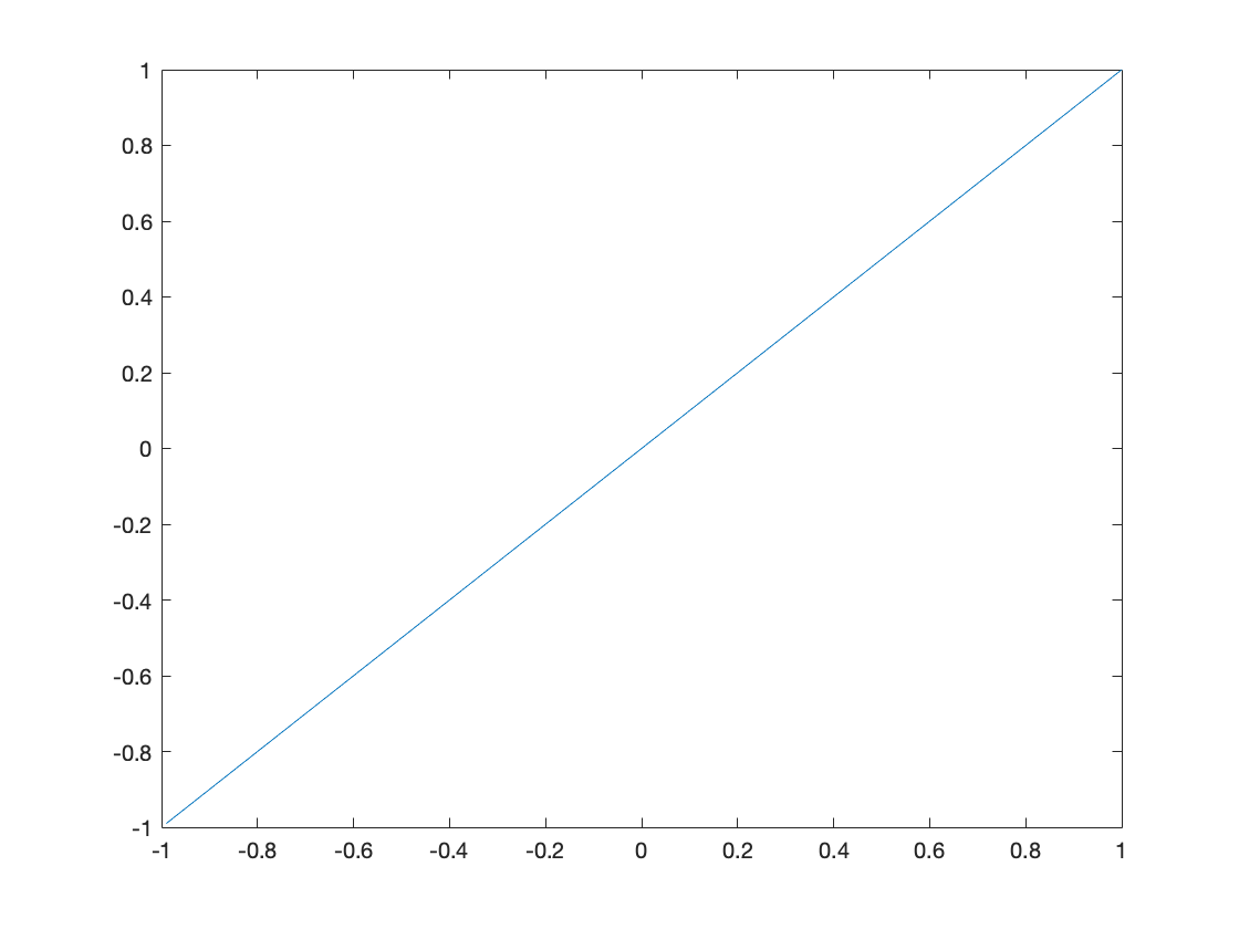
plot(x,real(ifft( N * X))); % Plot the function as computed via discrete fourier transforms
drawnow;

figure(3);
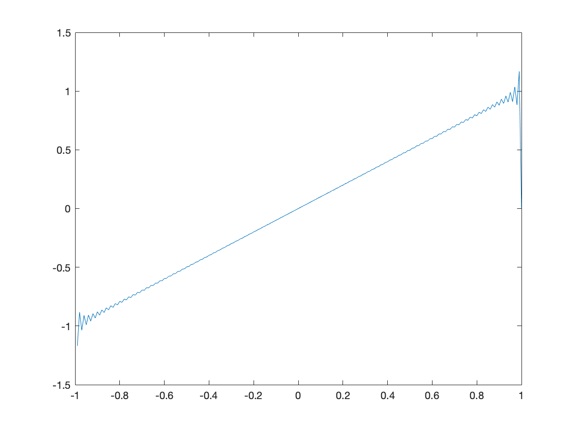
fourier = c .* fourier;
plot(x,real(N* ifft(fourier))); % Plot the function computed using the inverse fourier transform of the fourier coefficients
drawnow;

figure(4);
X = conj(c) .* X;
plot(y,real(fourier_val(X,y))); % Plot the truncated fourier series using the DFT approximation to the fourier coefficients

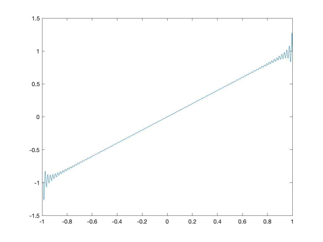
We notice here that Gibbs phenomenon does not appear when we compute the inverse discrete fourier transform of the discrete fourier transform. On the one hand this isn't surprising at all - after all the discrete fourier transform is a bijective on sequence space. However it does show one of the interesting behaviours of discrete fourier transforms - they include information about higher frequency. This phenomenon is known as aliasing.

Spectral Methods using the Fast Fourier Transform

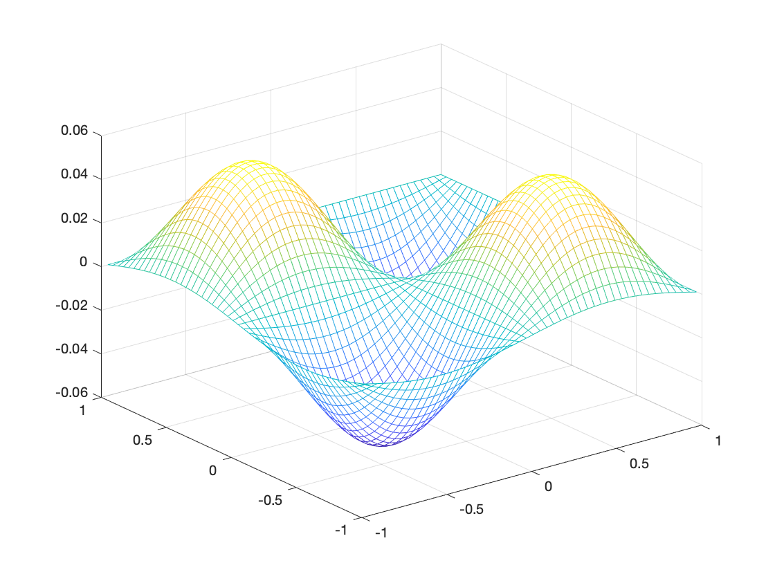
We are going to solve the Poisson equation using FFTs, $\nabla^2 u = f$ on $[-1, 1] \times [-1, 1]$ as in Lecture 13. In 2D frequency space this becomes $$ -\pi^2 ( k^2 + l^2) \hat{u}_{k,l} = \hat{f}_{k,l}$$. Therefore using Discrete Fourier Transforms we can write this algorithm as:

M = 50;

x = linspace(-1 + 2/M,1,M);
[X Y] = meshgrid(x,x);
g = @(x,y)(sin(x*pi).*sin(y*pi));

f  = g( X, Y );


f_f = fft2(f);
u = zeros(size(f_f));
four_coef = [0:M/2 (-M/2+1):-1];

for i = 1:numel(four_coef)
    for j = 1:numel(four_coef)
        if i+j > 2
            u(i,j) = -f_f(i,j)/(pi^2*(four_coef(i)^2+four_coef(j)^2));
        end
    end
end

u = ifft2(u);
figure(5);
mesh(X, Y, real(u));

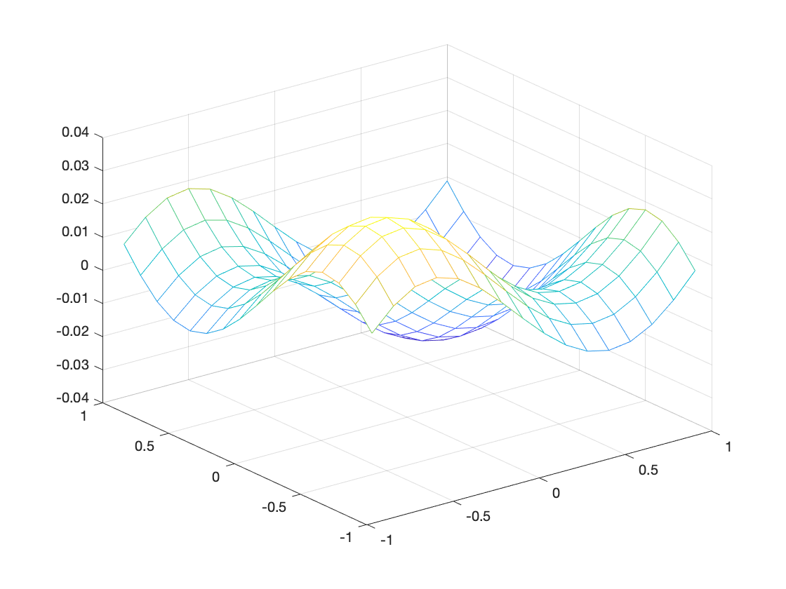
Solving a General Second Order PDE

Following the notes for Lecture 13, we wish to solve $\nabla^{T}(a \nabla u) = f$ on the same domain. Using the same set up as the notes we wish to solve:

$- \pi^2 \sum \left [ (km + ln) \hat{a}_{k-m, l-n} \hat{u}_{m,n} \right ] = \hat{f}_{k,l}$

Solving the numerical analysis problem from 2011 Part II Paper 4 ( $f = \sin \pi x + \sin \pi y, a = 3 + \cos \pi x + \cos \pi y$) can be done using MATLAB as follows:

M = 16;
x = linspace(-1 + 2/M,1,M);
[X Y] = meshgrid(x,x);
g = @(x,y)(sin(x*pi) + sin(y*pi));
a_fun = @(x,y)(3 + cos(pi*x) + cos(pi*y)+3);

f = g ( X, Y );
f = fft2(f);
a = a_fun ( X, Y );
a = fft2(a)/M^2;
four_coef = [0:M/2 (-M/2+1):-1];

A = zeros(M,M,M,M);
for k = 1:M, for l = 1:M, for m = 1:M, for n = 1:M
    if k-m <= M/2 && k-m >= 0
        if l - n <= M/2 && l-n >= 0
            A(m,n,k,l) = (four_coef(k)*four_coef(m)+four_coef(l)*four_coef(n))*a(k-m+1,l-n+1);
        elseif l-n >= -M/2+1 && l-n < 0
            A(m,n,k,l) = (four_coef(k)*four_coef(m)+four_coef(l)*four_coef(n))*a(k-m+1,M+1+(l-n));
        else
            A(m,n,k,l) = 0;
        end
    elseif k-m >= -M/2+1 && k-m < 0
        if l - n <= M/2  && l-n >= 0
            A(m,n,k,l) = (four_coef(k)*four_coef(m)+four_coef(l)*four_coef(n))*a(M+1+(k-m),l-n+1);
        elseif l-n >= -M/2+1 && l-n < 0
            A(m,n,k,l) = (four_coef(k)*four_coef(m)+four_coef(l)*four_coef(n))*a(M+1+(k-m),M+1+(l-n));
        else
            A(m,n,k,l) = 0;
        end
    else
        A(m,n,k,l) = 0;
    end
end,end,end,end;

B = reshape(A, M^2, M^2);

B(1,1) = 1;
f_vec = reshape(f,[],1);
f_vec(1) = 0;

u = B\f_vec;
u = -reshape(u,M,M)/pi^2;
u = ifft2(u);
figure(6);
mesh(X,Y, real(u));

Code

Published with MATLAB® R2017a