

Runge-Kutta (RK) Methods
This module is intended to be read after the relevant lectures.
Contents
Introduction: Beyond quadrature
FUNDAMENTAL POINT: RK methods are inspired by quadrature.
Suppose the equation of interest is 
RHS a function of time only
If the right-hand side is a function of  only (and NOT of
  ) then the problem reduces to a simple integration, for which quadrature is appropriate. Consider
  with
with  ; the exact solution is
  . We have the following numerical results using the common RK4 scheme detailed in [1] (with
  ):
):
a=10;
rk_test(@(t,y)(a*exp(-a*t)),@(t)(1-exp(-a*t)),0,0,3,7);
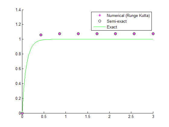
The 'semi-exact' scheme is RK except that it cheats slightly by using the exact whenever we evaluate  .
.
Here however, is independent of and so the 'semi-exact' scheme agrees with the RK scheme exactly. Due to the error in the quadrature scheme on which the RK scheme is based, both solutions deviate from the exact solution (we use a large step size for illustration).
The general case
However, in the general case,  varies with ; now we cannot simply use a quadrature rule, because we don't know the values of
  to use in between the current and next time-steps!
The basic idea of RK
The essence of RK methods is generalising quadrature by devising appropriate approximations to  . Of course, the devil is in the details, and the approximations are of a certain fixed form as explained in lectures.
The outcome is that there are two approximations in RK methods:
- The underlying quadrature approximation.
- The approximation to used for .
A comparison in the general case
We consider now  with
with  . The exact solution is
  . With
  :
:
b=5;
y0=1;
rk_test(@(t,y)(-b.*y^2),@(t)(1./(b.*t+1/y0)),y0,0,3,11);
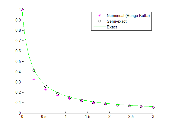
In this case, we can see the error introduced by approximating .
Fortunately, the approximations are chosen such that the method has order 4, so the error decays quite quickly with step size. (Again, we have chosen a large step size for illustration - otherwise the various solutions become indistinguishable!)
REFERENCES
[1]: (Wikipedia) Runge-Kutta Methods
Code
- rk_test.m (Function used above)