1 Geodesics in Spacetime
Classical theories of physics involve two different objects: particles and fields. The fields tell the particles how to move, and the particles tell the fields how to sway. For each of these, we need a set of equations.
In the theory of electromagnetism, the swaying of the fields is governed by the Maxwell equations, while the motion of test particles is dictated by the Lorentz force law. Similarly, for gravity we have two different sets of equations. The swaying of the fields is governed by the Einstein equations, which describe the bending and curving of spacetime. We will need to develop some mathematical machinery before we can describe these equations; we will finally see them in Section 4.
Our goal in this section is to develop the analog of the Lorentz force law for gravity. As we will see, this is the question of how test particles move in a fixed, curved spacetime. Along the way, we will start to develop some language to describe curved spacetime. This will sow some intuition which we will then make mathematically precise in later sections.
The Principle of Least Action
Our tool of choice throughout these lectures is the action. The advantage of the action is that it makes various symmetries manifest. And, as we shall see, there are some deep symmetries in the theory of general relativity that must be maintained. This greatly limits the kinds of equations which we can consider and, ultimately, will lead us inexorably to the Einstein equations.
We start here with a lightening review of the principle of least action. (A more detailed discussion can be found in the lectures on Classical Dynamics.) We describe the position of a particle by coordinates where, for now, we take for a particle moving in three-dimensional space. Importantly, there is no need to identify the coordinates with the axes of Euclidean space; they could be any coordinate system of your choice.
We want a way to describe how the particle moves between fixed initial and final positions,
| (1.2) |
To do this, we consider all possible paths , subject to the boundary conditions above. To each of these paths, we assign a number called the action . This is defined as
where the function is the Lagrangian which specifies the dynamics of the system. The action is a functional; this means that you hand it an entire function worth of information, , and it spits back only a single number.
The principle of least action is the statement that the true path taken by the particle is an extremum of . Although this is a statement about the path as a whole, it is entirely equivalent to a set of differential equations which govern the dynamics. These are known as the Euler-Lagrange equations.
To derive the Euler-Lagrange equations, we think about how the action changes if we take a given path and vary it slightly,
We need to keep the end points of the path fixed, so we demand that . The change in the action is then
where we have integrated by parts to go to the second line. The final term vanishes because we have fixed the end points of the path. A path is an extremum of the action if and only if for all variations . We see that this is equivalent to the Euler-Lagrange equations
| (1.3) |
Our goal in this section is to write down the Lagrangian and action which govern particles moving in curved space and, ultimately, curved spacetime.
1.1 Non-Relativistic Particles
Let’s start by forgetting about special relativity and spacetime and focus instead on the non-relativistic motion of a particle in curved space. Mathematically, these spaces are known as manifolds, and the study of curved manifolds is known as Riemannian geometry. However, for much of this section we will dispense with any formal mathematical definitions and instead focus attention on the physics.
1.1.1 The Geodesic Equation
We begin with something very familiar: the non-relativistic motion of a particle of mass in flat Euclidean space . For once, the coordinates actually are the usual Cartesian coordinates. The Lagrangian that describes the motion is simply the kinetic energy,
| (1.4) |
The Euler-Lagrange equations (1.3) applied to this Lagrangian simply tell us that , which is the statement that free particles move at constant velocity in straight lines.
Now we want to generalise this discussion to particles moving on a curved space. First, we need a way to describe curved space. We will develop the relevant mathematics in Sections 2 and 3 but here we offer a simple perspective. We describe curved spaces by specifying the infinitesimal distance between any two points, and , known as the line element. The most general form is
| (1.5) |
where the matrix is called the metric. The metric is symmetric: since the anti-symmetric part drops out of the distance when contracted with . We further assume that the metric is positive definite and non-degenerate, so that its inverse exists. The fact that is a function of the coordinates simply tells us that the distance between the two points and depends on where you are.
Before we proceed, a quick comment: it matters in this subject whether the indices are up or down. We’ll understand this better in Section 2 but, for now, remember that coordinates have superscripts while the metric has two subscripts.
We’ll see plenty of examples of metrics in this course. Before we introduce some of the simpler metrics, let’s first push on and understand how a particle moves in the presence of a metric. The Lagrangian governing the motion of the particle is the obvious generalization of (1.4)
| (1.6) |
It is a simple matter to compute the Euler-Lagrange equations (1.3) that arise from this action. It is really just an exercise in index notation and, in particular, making sure that we don’t inadvertently use the same index twice. Since it’s important, we proceed slowly. We have
where we’ve been careful to relabel the indices on the metric so that the index matches on both sides. Similarly, we have
Putting these together, the Euler-Lagrange equation (1.3) becomes
Because the term in brackets is contracted with , only the symmetric part contributes. We can make this obvious by rewriting this equation as
| (1.7) |
Finally, there’s one last manoeuvre: we multiply the whole equation by the inverse metric, , so that we get an equation of the form . We denote the inverse metric simply by raising the indices on the metric, from subscripts to superscripts. This means that the inverse metric is denoted . By definition, it satisfies
Finally, taking the opportunity to relabel some of the indices, the equation of motion for the particle is written as
| (1.8) |
where
| (1.9) |
These coefficients are called the Christoffel symbols. By construction, they are symmetric in their lower indicies: . They will play a very important role in everything that follows. The equation of motion (1.8) is the geodesic equation and solutions to this equation are known as geodesics.
A Trivial Example: Flat Space Again
Let’s start by considering flat space . Pythagoras taught us how to measure distances using his friend, Descartes’ coordinates,
| (1.10) |
Suppose that we work in polar coordinates rather than Cartestian coordinates. The relationship between the two is given by
In polar coordinates, the infinitesimal distance between two points can be simply derived by substituting the above relations into (1.10). A little algebra yields,
In this case, the metric (and therefore also its inverse) are diagonal. They are
where the matrix components run over . From this we can easily compute the Christoffel symbols. The non-vanishing components are
| (1.11) |
There are some important lessons here. First, does not necessarily mean that the space is curved. Non-vanishing Christoffel symbols can arise, as here, simply from a change of coordinates. As the course progresses, we will develop a diagnostic to determine whether space is really curved or whether it’s an artefact of the coordinates we’re using.
The second lesson is that it’s often a royal pain to compute the Christoffel symbols using (1.9). If we wished, we could substitute the Christoffel symbols into the geodesic equation (1.8) to determine the equations of motion. However, it’s typically easier to revert back to the original action and determine the equations of motion directly. In the present case, we have
| (1.12) |
and the resulting Euler-Lagrange equations are
| (1.13) |
These are nothing more than the equations for a straight line described in polar coordinates. The quickest way to extract the Christoffel symbols is usually to compute the equations of motion from the action, and then compare them to the geodesic equation (1.8), taking care of the symmetry properties along the way.
A Slightly Less Trivial Example:
The above description of in polar coordinates allows us to immediately describe a situation in which the space is truly curved: motion on the two-dimensional sphere . This is achieved simply by setting the radial coordinate to some constant value, say . We can substitute this constraint into the action (1.12) to get the action for a particle moving on the sphere,
Similarly, the equations of motion are given by (1.13), with the restriction and . The solutions are great circles, which are geodesics on the sphere. To see this in general is a little complicated, but we can use the rotational invariance to aid us. We rotate the sphere to ensure that the starting point is and the initial velocity is . In this case, it is simple to check that solutions take the form and for some , which are great circles running around the equator.
1.2 Relativistic Particles
Having developed the tools to describe motion in curved space, our next step is to consider the relativistic generalization to curved spacetime. But before we get to this, we first need to see how to extend the Lagrangian method to be compatible with special relativity. An introduction to special relativity can be found in the lectures on Dynamics and Relativity.
1.2.1 A Particle in Minkowski Spacetime
Let’s start by considering a particle moving in Minkowski spacetime . We’ll work with Cartestian coordinates and the Minkowski metric
The distance between two neighbouring points labelled by and is then given by
Pairs of points with are said to be timelike separated; those for which are spacelike separated; and those for which are said to be lightlike separated or, more commonly, null.
Consider the path of a particle through spacetime. In the previous section, we labelled positions along the path using the time coordinate for some inertial observer. But to build a relativistic description of the particle motion, we want time to sit on much the same footing as the spatial coordinates. For this reason, we will introduce a new parameter – let’s call it – which labels where we are along the worldline of the trajectory. For now it doesn’t matter what parameterisation we choose; we will only ask that increases monotonically along the trajectory. We’ll label the start and end points of the trajectory by and respectively, with and .
The action for a relativistic particle has a nice geometric interpretation: it extremises the distance between the starting and end points in Minkowski space. A particle with rest mass follows a timelike trajectory, for which any two points on the curve have . We therefore take the action to be
| (1.14) | |||||
The coefficients in front ensure that the action has dimensions as it should. (The action always has the same dimensions as . If you work in units with then the action should be dimensionless.)
The action (1.14) has two different symmetries, with rather different interpretations.
-
•
Lorentz Invariance: Recall that a Lorentz transformation is a rotation in spacetime. This acts as
(1.15) where the matrix obeys , which is the definition of a Lorentz transformation, encompassing both rotations in space and boosts. Equivalently, . This is a symmetry in the sense that if we find a solution to the equations of motion, then we can act with a Lorentz transformation to generate a new solution.
-
•
Reparameterisation invariance: We introduced as an arbitrary parameterisation of the path. But we don’t want the equations of motion to depend on this choice. Thankfully all is good, because the action itself does not depend on the choice of parameterisation. To see this, suppose that we picked a different parameterisation of the path, , related to the first parameterization by a monotonic function . Then we could equally as well construct an action using this new parameter, given by
As promised, the action takes the same form regardless of whether we choose to parameterise the path in terms of or . This is reparameterisation invariance.
This is not a symmetry, in the sense that it does not generate new solutions from old ones. Instead, it is a redundancy in the way we describe the system. It is similar to the gauge “symmetry” of Maxwell and Yang-Mills theory which, despite the name, is also a redundancy rather than a symmetry.
It is hard to overstate the importance of the concept of reparameterisation invariance. A major theme of these lectures is that our theories of physics should not depend on the way we choose to parameterise them. We’ll see this again when we come to describe the field equations of general relativity. For now, we’ll look at a couple of implications of reparameterisation on the worldline.
Proper Time
Because the action is independent of the parameterisation of the worldline, the value of the action evaluated between two points on a given path has an intrinsic meaning. We call this value proper time. For a given path , the proper time between two points, say and , is
| (1.16) |
From our first foray into Special Relativity, we recognise this as the time experienced by the particle itself.
Identifying the action with the proper time means that the particle takes a path that extremises the proper time. In Minkowski space, it is simple to check that the proper time between two timelike-separated points is maximised by a straight line, a fact known as the twin paradox.
1.2.2 Why You Get Old
There’s a crucial difference between moving in Euclidean space and moving in Minkowski spacetime. You’re not obliged to move in Euclidean space. You can just stop if you want to. In contrast, you can never stop moving in a timelike direction in Minkowski spacetime. You will, sadly, always be dragged inexorably towards the future.
Any relativistic formulation of particle mechanics must capture this basic fact. To see how it arises from the action (1.14), we can compute the momentum conjugate to ,
| (1.17) |
with . For the action , we have
| (1.18) |
But not all four components of the momentum are independent. To see this, we need only compute the square of the 4-momentum to find
| (1.19) |
Rearranging gives
In particular, we see that we must have : the particle is obliged to move in the time direction.
Part of this story is familiar. The condition (1.19) is closely related to the usual condition on the 4-momentum that we met in our earlier lectures on Special Relativity. There, we defined the 4-velocity and 4-momentum as
This is a special case of (1.17), where we choose to parameterise the worldline by the proper time itself. The definition of the proper time (1.16) means that . Comparing to the canonical momentum (1.18), we see that it coincides with the older definition above: .
However, part of this story is likely unfamiliar. Viewed from the perspective of classical dynamics, it is perhaps surprising to see that the momenta are not all independent. After all, this didn’t arise in any of the examples of Lagrangians that we met in our previous course on Classical Dynamics. This novel feature can be traced to the existence of reparameterisation invariance, meaning that there was a redundancy in our original description. Indeed, whenever theories have such a redundancy there will be some constraint analogous to (1.19). (In the context of electromagnetism, this constraint is called Gauss law.)
There is another way to view this. The relativistic action (1.14) appears to have four dynamical degrees of freedom, . This should be contrasted with the three degrees of freedom in the non-relativistic action (1.6). Yet the number of degrees of freedom is one of the most basic ways to characterise a system, with physical consequences such as the heat capacity of gases. Why should we suddenly increase the number of degrees of freedom just because we want our description to be compatible with special relativity? The answer is that, because of reparameterisation invariance, not all four degrees of freedom are physical. To see this, suppose that you solve the equations of motion to find the path (as we will do shortly). In most dynamical systems, each of these four functions would tell you something about the physical trajectory. But, for us, reparameterisation invariance means that there is no actual information in the value of . To find the physical path, we should eliminate to find the relationship between the . The net result is that the relativistic system only has three physical degrees of freedom after all.
As an example, we are perfectly at liberty to choose the parameterisation of the path to coincide with the time for some inertial observer: . The action (1.14) then becomes
| (1.20) |
where here . This is the action for a relativistic particle in some particular inertial frame, which exhibits the famous factor
that is omnipresent in formulae in special relativity. We now see clearly that the action has only three degrees of freedom, . However, the price we’ve paid is that the Lorentz invariance (1.15) is now rather hidden, since space and time sit on very different footing.
1.2.3 Rediscovering the Forces of Nature
So far, we’ve only succeeded in writing down the action for a free relativistic particle (1.14). We would now like to add some extra terms to the action to describe a force acting on the particle. In the non-relativistic context, we do this by adding a potential
However, now we want to write down an action for a relativistic particle that depends on . But it’s crucial that we retain reparameterisation invariance, since we want to keep the features that this brings. This greatly limits the kind of terms that we can add to the action. It turns out that there are two, different ways to introduce forces that preserve our precious reparameterisations.
Rediscovering Electromagnetism
Rather than jumping straight into the reparameterisation invariant action (1.14), we instead start by modifying the action (1.20). We’ll then try to guess a reparameterisation invariant form which gives the answer we want. To this end, we consider
and ask: how can this come from a reparameterisation invariant action?
We can’t just add a term to the relativistic action (1.14); this is not invariant under reparameterisations. To get something that works, we have to find a way to cancel the Jacobian factor that comes from reparameterisations of the measure. One option that we could explore is to introduce a term linear in . But then, to preserve Lorentz invariance, we need to contract the index on with something. This motivates us to introduce four functions of the spacetime coordinates . We then write the action
| (1.21) |
where is some number, associated to the particle, that characterises the strength with which it couples to the new term . It’s simple to check that the action (1.21) does indeed have reparameterisation invariance.
To understand the physics of this new term, we again pick the worldline parameter to coincide with the time of some inertial observer, so that . If we write , then we find
We see that the term gives us a potential of the kind we wanted. But Lorentz invariance means that this is accompanied by an additional term. We have, of course, met both of these terms previously: they describe a particle of electric charge moving in the background of an electromagnetic field described by gauge potentials and . In other words, we have rediscovered the Lorentz force law of electromagnetism.
There is a slight generalisation of this argument, in which the particle carries some extra internal degrees of freedom, that results in the mathematical structure of Yang-Mills, the theory that underlies the weak and strong nuclear force. You can read more about this in the lecture notes on Gauge Theory.
Rediscovering Gravity
To describe the force of gravity, we must make a rather different modification to our action. This time we consider the generalisation of (1.20) given by the action
| (1.22) |
If we Taylor expand the square-root, assuming that and that , then the leading terms give
| (1.23) |
The first term is an irrelevant constant. (It is the rest mass energy of the particle.) But the next two terms describe the non-relativistic motion of a particle moving in a potential .
Why should we identify this potential with the force of gravity, rather than some other random force? It’s because the strength of the force is necessarily proportional to the mass of the particle, which shows up as the coefficient in the term. This is the defining property of gravity.
In fact, something important but subtle has emerged from our simple discussion: the same mass appears in both the kinetic term and the potential term. In the framework of Newtonian mechanics there is no reason that these coefficients should be the same. Indeed, careful treatments refer to the coefficient of the kinetic term as the inertial mass and the coefficient of the potential term as the gravitational mass . It is then an experimentally observed fact that
| (1.24) |
to astonishing accuracy (around ). This is known as the equivalence principle. But our simple-minded discussion above has offered a putative explanation for the equivalence principle, since the mass sits in front of the entire action (1.22), ensuring that both terms have the same origin.
An aside: you might wonder why the function does not scale as, say, , in which case the potential that arises in (1.23) would appear to be independent of . This is not allowed. This is because the mass is a property of the test particle whose motion we’re describing. Meanwhile the potential is some field set up by the background sources, and should be independent of , just as is independent of the charge of the test particle.
The equality (1.24) is sometimes called the weak equivalence principle. A stronger version, known as the Einstein equivalence principle says that in any metric there exist local inertial frames. This is the statement that you can always find coordinates so that, in some small patch, the metric looks like Minkowski space, and there is no way to detect the effects of the gravitational field. We will describe this more below and again in Section 3.3.2.
Finally, we ask: how can we write down a reparameterisation invariant form of the action (1.22)? To answer this, note that the 1 in came from the term in the action. If we want to turn this into , then we should promote to a function of . But if we’re going to promote to a function, we should surely do the same to all metric components. This means that we introduce a curved spacetime metric
The metric is a symmetric matrix, which means that it is specified by 10 functions. We can then write down the reparameterisation invariant action
This describes a particle moving in curved spacetime.
In general, the components of the metric will be determined by the Einstein field equations. This is entirely analogous to the way in which the gauge potential in (1.21) is determined by the Maxwell equation. We will describe the Einstein equations in Section 4. However, even before we get to the Einstein equations, the story above tells us that, for weak gravitational fields where the Newtonian picture is valid, we should identify
| (1.25) |
where is the Newtonian gravitational field.
1.2.4 The Equivalence Principle
A consequence of the weak equivalence principle (1.24) is that it’s not possible to tell the difference between constant acceleration and a constant gravitational field. Suppose, for example, that you one day wake up to find yourself trapped inside a box that looks like an elevator. The equivalence principle says that there’s no way tell whether you are indeed inside an elevator on Earth, or have been captured by aliens and are now in the far flung reaches of the cosmos in a spaceship, disguised as an elevator, and undergoing constant acceleration. (Actually there are two ways to distinguish between these possibilities. One is common sense. The other is known as tidal forces and will be described below.)
Conversely, if you wake in the elevator to find yourself weightless, the equivalence principle says that there is no way to tell whether the engines on your spaceship have turned themselves off, leaving you floating in space, or whether you are still on Earth, plummeting towards certain death. Both of these are examples of inertial frames.
We can see how the equivalence principle plays out in more detail in the framework of spacetime metrics. We will construct a set of coordinates adapted to a uniformly accelerating observer. We’ll see that, in these coordinates, the metric takes the form (1.25) but with a linear gravitational potential of the kind that we would invoke for a constant gravitational force.
First we need to determine the trajectory of a constantly accelerating observer. This was a problem that we addressed already in our first lectures on Special Relativity (see Section 7.4.6 of those notes). Here we give a different, and somewhat quicker, derivation.
We will view things from the perspective of an inertial frame, with coordinates . The elevator will experience a constant acceleration in the direction. We want to know what this looks like in the inertial frame; clearly the trajectory is not just since this would soon exceed the speed of light. Instead we need to be more careful.
Recall that if we do a boost by , followed by a boost by , the resulting velocity is
This motivates us to define the rapidity , defined in terms of the velocity by
The rapidity has the nice property that is adds linearly under successive boosts: a boost followed by a boost is the same as a boost .
A constant acceleration means that the rapidity increases linearly in time, where here “time” is the accelerating observer’s time, . We have and so, from the perspective of the inertial frame, the velocity of the constantly-accelerating elevator
To determine the relationship between the observer’s time and the time in the inertial frame, we use
where we’ve chosen the integration constant so that corresponds to . Then, to determine the distance travelled in the inertial frame, we use
where this time we’ve chosen the integration constant so that the trajectory passes through the origin. The resulting trajectory is a hyperbola in spacetime, given by
This trajectory is shown in red in Figure 1. As , the trajectory asymptotes to the straight lines . These are the dotted lines shown in the figure.
Now let’s consider life from the perspective of guy in the accelerating elevator. What are the natural coordinates that such an observer would use to describe events elsewhere in spacetime? Obviously, for events that happen on his own worldline, we can use the proper time . But we would like to extend the definition to assign a time to points in the whole space. Furthermore, we would like to introduce a spatial coordinate, , so that the elevator sits at . How to do this?
There is, it turns out, a natural choice of coordinates. First, we draw straight lines connecting the point to the point on the trajectory labelled by and declare that these are lines of constant ; these are the pink lines shown in the figure. Next we note that, for any given , there is a Lorentz transformation that maps the -axis to the pink line of constant . We can use this to define the spatial coordinate . The upshot is that we have a map between coordinates in the inertial frame and coordinates in the accelerating frame given by
| (1.26) |
As promised, the line coincides with the trajectory of the accelerating observer. Moreover, lines of constant are also hyperbolae.
The coordinates do not cover all of Minkowski space, but only the right-hand quadrant as shown in Figure 1. This reflects the fact that signals from some regions will never reach the guy in the elevator. This is closely related to the idea of horizons in general relativity, a topic we’ll look explore more closely in later sections.
Finally, we can look at the metric experienced by the accelerating observer, using coordinates and . We simply substitute the transformation (1.26) into the Minkowski metric to find
This is the metric of (some part of ) Minkowski space, now in coordinates adapted to an accelerating observer. These are known as Kottler-Möller coordinates. (They are closely related to the better known Rindler coordinates. We’ll see Rindler space again in Section 6.1.2 when we study the horizon of black holes. ) The spatial part of the metric remains flat, but the temporal component is given by
where the is simply , but we’ve hidden it because it is sub-leading in . If we compare this metric with the expectation (1.25), we see that the accelerated observer feels an effective gravitational potential given by
This is the promised manifestation of the equivalence principle: from the perspective of an uniformly accelerating observer, the acceleration feels indistinguishable from a linearly increasing gravitational field, corresponding to a constant gravitational force.
The Einstein Equivalence Principle
The weak equivalence principle tells us that uniform acceleration is indistinguishable from a uniform gravitational field. In particular, there is a choice of inertial frame (i.e. free-fall) in which the effect of the gravitational field vanishes. But what if the gravitational field is non-uniform?
The Einstein equivalence principle states that there exist local inertial frames, in which the effects of any gravitational field vanish. Mathematically, this means that there is always a choice of coordinates — essentially those experienced by a freely falling observer – which ensures that the metric looks like Minkowski space about a given point. (We will exhibit these coordinates and be more precise about their properties in Section 3.3.2.) The twist to the story is that if the metric looks like Minkowski space about one point, then it probably won’t look like Minkowski space about a different point. This means that if you can do experiments over an extended region of space, then you can detect the presence of non-uniform gravitational field.
To illustrate this, let’s return to the situation in which you wake, weightless in an elevator, trying to figure out if you’re floating in space or plummeting to your death. How can you tell?
Well, you could wait and find out. But suppose you’re impatient. The equivalence principle says that there is no local experiment you can do that will distinguish between these two possibilities. But there is a very simple “non-local” experiment: just drop two test masses separated by some distance. If you’re floating in space, the test masses will simply float there with you. Similarly, if you’re plummeting towards your death then the test masses will plummet with you. However, they will each be attracted to the centre of the Earth which, for two displaced particles, is in a slightly different direction as shown in Figure 2. This means that the trajectories followed by the particles will slightly converge. From your perspective, this will mean that the two test masses will get closer. This is not due to their mutual gravitational attraction. (The fact they’re test masses means we’re ignoring this). Instead, it is an example of a tidal force that signifies you’re sitting in a non-uniform gravitational field. We will meet the mathematics behind these tidal forces in Section 3.3.4.
1.2.5 Gravitational Time Dilation
Even before we solve the Einstein equations, we can still build some intuition for the spacetime metric. As we’ve seen, for weak gravitational fields , we should identify the temporal component of the metric as
| (1.27) |
This is telling us something profound: there is a connection between time and gravity.
To be concrete, we’ll take the Newtonian potential that arises from a spherical object of mass ,
The resulting shift in the spacetime metric means that an observer sitting at a fixed distance will measure a time interval,
This means that if an asymptotic observer, at , measures time , then an observer at distance will measure time given by
We learn that time goes slower in the presence of a massive, gravitating object.
We can make this more quantitative. Consider two observers. The first, Alice, is relaxing with a picnic on the ground at radius . The second, Bob, is enjoying a romantic trip for one in a hot air balloon, a distance higher. The time measured by Bob is
where we’ve done a double expansion, assuming both and . If the hot air balloon flies a distance above the ground then, taking the radius of the Earth to be , the difference in times is of order . This means that, over the course of a day, Bob ages by an extra seconds or so.
This effect was first measured by Hafele and Keating in the 1970s by flying atomic clocks around the world on commercial airlines, and has since been repeated a number of times with improved accuracy. In all cases the resultant time delay, which in the experiments includes effects from both special and general relativity, was in agreement with theoretical expectations.
The effect is more pronounced in the vicinity of a black hole. We will see in Section 1.3 that the closest distance that an orbiting planet can come to a black hole is . (Such orbits are necessarily highly elliptical.) In this case, someone on the planet experiences time at the rate , compared to an asymptotic observer at . This effect, while impressive, is unlikely to make a really compelling science fiction story. For more dramatic results, our bold hero would have to fly her spaceship close to the Schwarzschild radius , later returning to to find herself substantially younger than the friends and family she left behind.
Gravitational Redshift
There is another measurable consequence of the gravitational time dilation. To see this, let’s return to Alice on the ground and Bob, above, in his hot air balloon. Bob is kind of annoying and starts throwing peanuts at Alice. He throws peanuts at time intervals . Alice receives these peanuts (now travelling at considerable speed) at time intervals where, as above,
We have , so and, hence, . In other words, Alice receives the peanuts at a higher frequency than Bob threw them.
The story above doesn’t only hold for peanuts. If Bob shines light down at Alice with frequency , then Alice will receive it at frequency given by
This is a higher frequency, , or shorter wavelength. We say that the light has been blueshifted. In contrast, if Alice shines light up at Bob, then the frequency decreases, and the wavelength is stretched. In this case, we say that the light has been redshifted as it escapes the gravitational pull. This effect was measured for the first time by Pound and Rebka in 1959, providing the first earthbound precision test of general relativity.
There is a cosmological counterpart of this result, in which light is redshifted in a background expanding space. You can read more about this in the lectures on Cosmology.
1.2.6 Geodesics in Spacetime
So far, we have focussed entirely on the actions describing particles, and have have yet to write down an equation of motion, let alone solve one. Now it’s time to address this.
We work with the relativistic action for a particle moving in spacetime
| (1.28) |
with . This is similar to the non-relativistic action that we used in Section 1.1.1 when we first introduced geodesics. It differs by the square-root factor. As we now see, this introduces a minor complication.
To write down Euler-Lagrange equations, we first compute
The equations of motion are then
This is almost the same as the equations that led us to the geodesics in Section 1.1.1. There is just one difference: the differentiation can hit the , giving an extra term beyond what we found previously. This can be traced directly to the fact we have a square-root in our original action.
Life would be much nicer if there was some way to ignore this extra term. This would be true if, for some reason, we could set
Happily, this is within our power. We simply need to pick a choice of parameterisation of the worldline to make it hold! All we have to do is figure out what parameterisation makes this work.
In fact, we’ve already met the right choice. Recall that the proper time is defined as (1.16)
| (1.30) |
This means that, by construction,
If we then choose to parameterise the path by itself, the Lagrangian is
The upshot of this discussion is that if we parameterise the worldline by proper time then is a constant and, in particular, . In fact this holds for any parameter related to proper time by
with and constants. These are said to be affine parameters of the worldline.
Whenever we pick such an affine parameter to label the worldline of a particle, the right-hand side of the equation of motion (1.29) vanishes. In this case, we are left with the obvious extension of the geodesic equation (1.8) to curved spacetime
| (1.31) |
where the Christoffel symbols are given, as in (1.9), by
| (1.32) |
A Useful Trick
We’ve gone on something of a roundabout journey. We started in Section 1.1.1 with a non-relativistic action
and found that it gives rise to the geodesic equation (1.8).
However, to describe relativistic physics in spacetime, we’ve learned that we need to incorporate reparameterisation invariance into our formalism resulting in the action
Nonetheless, when we restrict to a very particular parameterisation – the proper time – we find exactly the same geodesic equation (1.31) that we met in the non-relativistic case.
This suggests something of a shortcut. If all we want to do is derive the geodesic equation for some metric, then we can ignore all the shenanigans and simply work with the action
| (1.33) |
This will give the equations of motion that we want, provided that they are supplemented with the constraint
| (1.34) |
This is the requirement that the geodesic is timelike, with the proper time. This constraint now drags the particle into the future. Note that neither (1.33) nor (1.34) depend on the mass of the particle. This reflects the equivalence principle, which tells us that each particle, regardless of its mass, follows a geodesic.
Moreover, we can also use (1.33) to calculate the geodesic motion of light, or any other massless particle. These follow null geodesics, which means that we simply need to replace (1.34) with
| (1.35) |
While the action is, as the name suggests, useful, you should be cautious in how you wield it. It doesn’t, as written, have the right dimensions for an action. Moreover, if you try to use it to do quantum mechanics, or statistical mechanics, then it might lead you astray unless you are careful in how you implement the constraint.
1.3 A First Look at the Schwarzschild Metric
Physics was born from our attempts to understand the motion of the planets. The problem was largely solved by Newton, who was able to derive Kepler’s laws of planetary motion from the gravitational force law. This was described in some detail in our first lecture course on Dynamics and Relativity.
Newton’s laws are not the end of the story. There are relativistic corrections to the orbits of the planets that can be understood by computing the geodesics in the background of a star.
To do this, we first need to understand the metric created by a star. This will be derived in Section 6. For now, we simply state the result: a star of mass gives rise to a curved spacetime given by
This is the Schwarzschild metric. The coordinates and are the usual spherical polar coordinates, with and .
We will have to be patient to fully understand all the lessons hiding within this metric. But we can already perform a few sanity checks. First, note that far from the star, as , it coincides with the Minkowski metric as it should. Secondly, the component is given by
which agrees with our expectation (1.25) with the usual Newtonian potential for an object of mass .
The Schwarzschild metric also has some strange things going on. In particular, the component diverges at where
is called the Schwarzschild radius. This is the event horizon of a black hole and will be explored more fully in Section 6. However, it turns out that space around any spherically symmetric object, such as a star, is described by the Schwarzschild metric, now restricted to , with the radius of the star.
In what follows we will mostly view the Schwarzschild metric as describing the spacetime outside a star, and treat the planets as test particles moving along geodesics in this metric. We will also encounter a number of phenomena that happen close to ; these are relevant only for black holes, since . However we will, for now, avoid any discussion of what happens if you venture past the event horizon.
1.3.1 The Geodesic Equations
Our first task is to derive the equations for a geodesic in the Schwarzschild background. To do this, we use the quick and easy method of looking at the action (1.33) for a particle moving in the Schwarzschild spacetime,
| (1.36) | |||||
with and .
When we solved the Kepler problem in Newtonian mechanics, we started by using the conservation of angular momentum to restrict the problem to a plane. We can use the same trick here. We first look at the equation of motion for ,
This tells us that if we kick the particle off in the plane, with , then it will remain there for all time. This is the choice we make.
We still have to compute the magnitude of the angular momentum. Like many conserved quantities, this follows naturally by identifying the appropriate ignorable coordinate. Recall that if the Lagrangian is independent of some specific coordinate then the Euler-Lagrange equations immediately give us a conserved quantity,
This is a baby version of Noether’s theorem.
The action (1.36) has two such ignorable coordinates, and . The conserved quantity associated to is the magnitude of the angular momentum, . (Strictly, the angular momentum per unit mass.) Restricting to the plane, we define this to be
| (1.37) |
where the factor of 2 on the left-hand side arises because the kinetic terms in (1.36) don’t come with the usual factor of . Meanwhile, the conserved quantity associated to is
| (1.38) |
The label is not coincidence: it should be interpreted as the energy of the particle (or, strictly, the energy divided by the rest mass). To see this, we look far away: as we have and we return to Minkowski space. Here, we know from our lectures on Special Relativity that . We then have as . But this is precisely the energy per unit rest mass of a particle in special relativity.
We should add to these conservation laws the constraint (1.34) which tells us that the geodesic is parameterised by proper time. Restricting to and , this becomes
| (1.39) |
If we now substitute in the expressions for the conserved quantities and , this constraint can be rewritten as
| (1.40) |
The effective potential includes the factor which we now write out in full,
| (1.41) |
Our goal is to solve for the radial motion (1.40). We subsequently use the expression (1.37) to solve for the angular motion and, in this way, determine the orbit.
1.3.2 Planetary Orbits in Newtonian Mechanics
Before we solve the full geodesic equations, it is useful to first understand how they differ from the equations of Newtonian gravity. To see this, we write
The non-relativistic limit is, roughly, . This means that we drop the final term in the potential that scales as . (Since is dimensionful, it is more accurate to say that we restrict to situations with .) Meanwhile, we expand the relativistic energy per unit mass in powers of ,
where is the non-relativistic energy and are terms suppressed by . Substituting these expressions into (1.40), we find
where is the non-relativistic potential which includes both the Newtonian gravitational potential and the angular momentum barrier,
These are precisely the equations that we solved in our first course on classical mechanics. (See Section 4.3 of the lectures on Dynamics and Relativity.) The only difference is that is parameterised by proper time rather than the observers time . However, these coincide in the non-relativistic limit that we care about.
We can build a lot of intuition for the orbits by looking at the potential , as shown in Figure 3. At large distances, the attractive gravitational potential dominates, while the angular momentum prohibits the particles from getting too close to the origin, as seen in the term which dominates at short distances. The potential has a minimum at
A particle can happily sit at for all time. This circular orbit always has energy , reflecting the fact that .
Alternatively, the particle could oscillate back and forth about the minima. This happens provided that so that the particle is unable to escape to . This motion describes an orbit in which the distance to the origin varies; we’ll see below that the shape of the orbit is an ellipse. Finally, trajectories with describe fly-bys, in which the particle approaches the star, but gets only so close before flying away never to be seen again.
The discussion above only tells us about the radial motion. To determine the full orbit, we need to use the angular momentum equation . Let’s remind ourselves how we solve these coupled equations. We start by employing a standard trick of working with the new coordinate
We then view this inverse radial coordinate as a function of the angular variable: . This works out nicely, since we have
where in the last equality, we’ve used angular momentum conservation (1.37) to write . Using this, we have
| (1.42) |
The equation giving conservation of energy is then
| (1.43) |
But this is now straightforward to solve. We choose to write the solution as
| (1.44) |
Back in our original radial variable, we have
| (1.45) |
This is the equation for a conic section, with the eccentricity given by
The shape of the orbit depends on . A particle with is not in a bound orbit, and traces out a hyperbola for and a parabola for . Planets, in contrast, have energy and, correspondingly, eccentricity . In this case, the orbits are ellipses.
To compare with the relativistic result later, we note an important feature of the Newtonian orbit: it does not precess. To see this, note that for our solution (1.45) the point at which the planet is closest to the origin – known as the perihelion – always occurs at the same point in the orbit.
1.3.3 Planetary Orbits in General Relativity
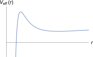
We now repeat this analysis for the full relativistic motion of a massive particle moving along a geodesic in the Schwarzschild metric. We have seen that the effective potential takes the form (1.41)
The relativistic correction scales as and changes the Newtonian story at short distances, since it ensures that the potential as . Indeed, the potential always vanishes at the Schwarzschild radius , with .
|
|
The potential takes different shapes, depending on the size of the angular momentum. To see this, we compute the critical points
| (1.46) |
If the discriminant is positive, then this quadratic equation has two solutions. This occurs when the angular momentum is suitably large.
In this case, the potential looks like the figure shown on the left. We call the two solutions to the quadratic equation (1.46), and with . The outermost solution is a minimum of the potential and corresponds to a stable circular orbit; the innermost solution is a maximum of the potential and corresponds to an unstable circular orbit.
As in the Newtonian setting, there are also non-circular orbits in which the particle oscillates around the minimum. However, there is no reason to think these will, in general, remain elliptical. We will study some of their properties below.
Note also that, in contrast to the Newtonian case, the angular momentum barrier is now finite: no matter how large the angular momentum, a particle with enough energy (in the form of ingoing radial velocity) will always be able to cross the barrier, at which point it plummets towards . We will say more about this in Section 6 when we discuss black holes.
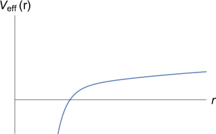
If the angular momentum is not large enough,
then the potential has no turning points and looks like the right-hand figure. In this case, there are no stable orbits; all particles will ultimately fall towards the origin.
The borderline case is . In this case the turning point is a saddle at
| (1.47) |
This is the innermost stable circular orbit. There can be no circular orbits at distances , although it is possible for the non-circular orbits to extend into distances .
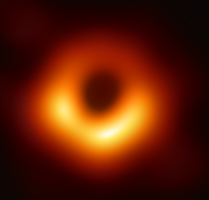
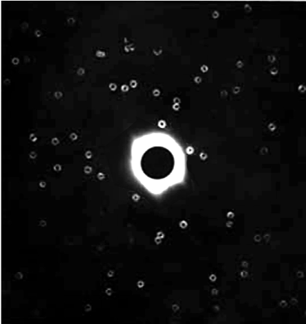
The innermost stable orbit plays an important role in black hole astrophysics, where it marks the inner edge of the accretion disc which surrounds the black hole. Roughly speaking, this is seen in the famous photograph captured by the Event Horizon Telescope. Here, the “roughly speaking” is because the light emitted from the accretion disc is warped in a dramatic fashion, so what we see is very different from what is there! (Furthermore, the black hole in the picture almost certainly rotating. This makes smaller than and the picture significantly harder to interpret.)
We could also ask: how close can a non-circular orbit get? This occurs in the limit , where a quick calculation shows that the maximum of tends to . This is the closest that any timelike geodesic can get if it wishes to return.
Perihelion Precession
To understand the orbits in more detail, we can attempt to solve the equations of motion. We follow our Newtonian analysis, introducing the inverse parameter and converting into . Our equation (1.40) becomes
This equation is considerably harder than our Newtonian orbit equation (1.43). To proceed, it’s simplest to first differentiate again with respect to . This gives
where we have assumed that , which means that we are neglecting the simple circular solution. The equation above differs from the analogous Newtonian equation by the final term (which indeed vanishes if we take ). There is no closed-form solution to this equation, but we can make progress by working perturbatively. To this end, we define the dimensionless parameter
and write the orbit equation as
| (1.48) |
We will assume and look for series solutions of the form
To leading order, we can ignore the terms proportional to on the right-hand-side of (1.48). This gives us an equation for which is identical to the Newtonian orbit
We now feed this back into the equation (1.48) to get an equation for ,
You can check that this is solved by
We could proceed to next order in , but the first correction will be sufficient for our purposes.
The interesting term is the in . This is not periodic in and it means that the orbit no longer closes: it sits at a different radial value at and . To illustrate this, we ask: when is the particle closest to origin? This is the perihelion of the orbit. It occurs when
Clearly this is solved by . The next solution is at where, due to our perturbative expansion, will be small. Expanding our expression above, and dropping terms of order and , we find the precession of the perihelion given by
| (1.49) |
For planets orbiting the Sun, the perihelion shift depends only on the angular momentum of the planet and the mass of the Sun, denoted . The latter is , corresponding to the length scale
If a planet on an almost-circular orbit of radius orbits the sun in a time , then the angular momentum (1.37) is
Recall that Kepler’s third law (which follows from the inverse square law) tells us that . This means that and, correspondingly, the perihelion shift (1.49) is proportional to . We learn that the effect should be more pronounced for planets closest to the Sun.
The closest planet to the Sun is Mercury which, happily, is also the only planet whose orbit differs significantly from a circle; it has eccentricity , the radius varying from to m. Mercury orbits the Sun once every 88 days but, in fact, we don’t need to use this to compute the angular momentum and precession. Instead, we can invoke the elliptic formula (1.45) which tells us that the minimum and maximum distance is given by
| (1.50) |
from which we get the precession
Plugging in the numbers gives . This is rather small. However, the perihelion precession is cumulative. Over a century, Mercury completes 415 orbits, giving the precession of per century.
The result above is quoted in radians. Astronomers prefer units of arcseconds, with 3600 arcseconds (denoted as ) in a degree and, of course, 360 degrees in radians. This means that . Our calculation from general relativity gives per century as the shift in the perihelion. This was one of the first successful predictions of the theory. Subsequently, the perihelion shift of Venus and Earth has been measured and is in agreement with the predictions of general relativity.
1.3.4 The Pull of Other Planets
The general relativistic contribution of per century is not the full story. In fact the observed perihelion shift of Mercury is much larger, at around . The vast majority of this is due to the gravitational force of other planets and can be understood entirely within the framework of Newtonian gravity. For completeness, we now give an estimate of these effects.
We start be considering the effect of single, heavy planet with mass , orbiting at a distance from the Sun. Of course, the 3-body problem in Newtonian gravity is famously hard. However, there is an approximation which simplifies the problem tremendously: we consider the outer planet to be a circular ring, with mass per unit length given by .
It’s not obvious that this is a good approximation. Each of the outer planets takes significantly longer to orbit the Sun than Mercury. This suggests for any given orbit of Mercury, it would be more appropriate to treat the position of the outer planets to be fixed. (For example, it takes Jupiter 12 years to orbit the Sun, during which time Mercury has completed 50 orbits.) This means that the perihelion shift of Mercury depends on the position of these outer planets and that’s a complicated detail that we’re happy to ignore. Instead, we want only to compute the total perihelion shift of Mercury averaged over a century. And for this, we may hope that the ring approximation, in which we average over the orbit of the outer planet first, suffices.
In fact, as we will see, the ring approximation is not particularly good: the calculation is non-linear and averaging over the position of the outer planet first does not commute with averaging over the orbits of Mercury. This means that we will get a ballpark figure for the perihelion precession of Mercury but, sadly, not one that is accurate enough to test relativity.
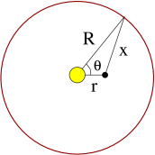
We would like to determine the Newtonian potential felt by a planet which orbits a star of mass and is surrounded, in the same plane, by a ring of density . The geometry is shown in the figure. Obviously, the potential (per unit mass) from the star is
We need to calculate the potential (per unit mass) from the ring. This is
| (1.51) |
We use the fact that Mercury is much closer to the Sun than the other planets and Taylor expand the integral in . To leading order we have
Dropping constant terms, we learn that the effective potential (per unit mass) experienced by Mercury is, to leading order,
where we’ve included the angular momentum barrier and the sum is over all the outer planets. In what follows, we must assume that the correction term is suitably small so that it doesn’t destabilise the existence of orbits. Obviously, this is indeed the case for Mercury.
Now we can follow our calculation for the perihelion precession in general relativity. Conservation of energy tells us
Working with everyone’s favourite orbit variable, , viewed as , the general relativistic equation (1.48) is replaced by
| (1.52) |
where this time our small dimensionless parameter is
where, in the second equality, we’ve used (1.50); here is the mass of the Sun, is the outermost radius of Mercury’s orbit, and is the eccentricity of Mercury’s orbit. We safely have and so we look for series solutions of the form
We’ve already met the leading order solution, with the eccentricity of the planet’s orbit. Feeding this into (1.52), we get an equation for the first correction
This equation is somewhat harder to solve than the general relativistic counterpart. To proceed, we will assume that the eccentricity is small, , and solve the equation to leading order in . Then this equation becomes
which has the solution
The precession of the perihelion occurs when
As in the relativistic computation, this is solved by and by where, to leading order, the shift of the perihelion is given by
with . Once again, we can put the numbers in. The mass of the Sun is . The formula is very sensitive to the radius of Mercury’s orbit: we use . The relevant data for the other planets is then
| Planet | Mass () | Distance () | |
|---|---|---|---|
| Venus | |||
|
Earth |
|||
|
Mars |
|||
| Jupiter | |||
| Saturn |
A quick glance at this table shows that the largest contributions come from Jupiter (because of its mass) and Venus (because of it proximity), with the Earth in third place. (The contributions from Uranus, Neptune and Pluto are negligible.)
Adding these contributions, we find radians per orbit. This corresponds to per century, significantly larger than the per century arising from general relativity but not close to the correct Newtonian value of .
Higher Order Contributions
Our analysis above gave us a result of per century for the perihelion shift of Mercury. A more precise analysis gives coming from the Newtonian pull of the other planets.
We made a number of different approximations in the discussion above. But the one that introduced the biggest error turns out to be truncating the ring potential (1.51) at leading order in . This, it turns out, is particularly bad for Venus since its orbit compared to Mercury is only . To do better, we can expand the potential (1.51) to higher orders. We have
An identical calculation to the one above now gives a corresponding perturbative expansion for the perihelion shift,
with the mean orbit of Mercury. The extra terms give significant contributions for Venus, and smaller for Earth. Using the value of and the slightly more accurate for Venus, the sum of the contributions gives radians per orbit, or per century, somewhat closer to the recognised value of per century but still rather short.
1.3.5 Light Bending
It is straightforward to extend the results above to determine the null geodesics in the Schwarzschild metric. We continue to use the equations of motion derived from in (1.36). But this time we replace the constraint (1.39) with the null version (1.35), which reads
The upshot is that we can again reduce the problem to radial motion,
| (1.53) |
but now with the effective potential (1.41) replaced by
A typical potential is shown in Figure 9. Note that, as , the potential asymptotes to zero from above, while as . The potential has a single maximum at
We learn that there is a distance, , at which light can orbit a black hole. This is known as the photon sphere. The fact that this sits on a maximum of the potential means that this orbit is unstable. In principle, focussing effects mean that much of the light emitted from an accretion disc around a non-rotating black hole emerges from the photon sphere. In practice, it seems likely that photograph of the Event Horizon Telescope does not have the resolution to see this.
The fate of other light rays depends on the relative value of their energy and angular momentum . To see this, note that the maximum value of the potential is
The physics depends on how this compares to the right-hand side of (1.53), . There are two possibilities
-
•
: In this case, the energy of light is lower than the angular momentum barrier. This means that light emitted from cannot escape to infinity; it will orbit the star, before falling back towards the origin. The flip side is that light coming from infinity will not fall into the star; instead it will bounce off the angular momentum barrier and return to infinity. In other words, the light will be scattered. We will compute this in more detail below.
-
•
: Now the energy of the light is greater than the angular momentum barrier. This means that light emitted from can escape to infinity. (We will see in Section 6 that this is only true for light in the region .) Meanwhile, light coming in from infinity is captured by the black hole and asymptotes to .
To understand the trajectories of light-rays in more detail, we again adopt the inverse parameter . The equation of motion (1.53) then becomes
If we now differentiate again, we get
| (1.54) |
We will again work perturbatively. First, suppose that we ignore the term on the right-hand side. We have
for constant . The meaning of this solution becomes clearer if we write it as : this is the equation of a horizontal straight line, a distance above the origin as shown by the dotted line in Figure 10. The distance is called the impact parameter.
We will solve the full equation (1.54) perturbatively in the small parameter
We then look for solutions of the form
We start with the straight line solution . At leading order, we then have
The general solution is
where the first two terms are the complimentary solution, with and integration constants. We pick them so that the initial trajectory at agrees with the straight line . This holds if we choose and , so that as . To leading order in , the solution is then
The question now is: at what angle does the particle escape to or, equivalently, ? Before we made the correction this happened at . Within our perturbative approach, we can approximate and to find that the particle escapes at
| (1.55) |
This light bending is known as gravitational lensing.
|

|
For the Sun, . If light rays just graze the surface, then the impact parameter coincides with the radius of the Sun, . This gives a scattering angle of radians, or .
There is a difficulty in testing this prediction: things behind the Sun are rarely visible. However, Nature is kind to us because the size of the moon as seen in the sky is more or less the same as the size of the Sun. (This random coincidence would surely make our planet a popular tourist destination for alien hippies if only it wasn’t such a long way to travel.) This means that during a solar eclipse the light from the Sun is blocked, allowing us to measure the positions of stars whose light passes nearby the Sun. This can then be compared to the usual positions of these stars.
This measurement was first carried out in May 1919, soon after cessation of war, in two expeditions led by Arthur Eddington, one to the island of Principe and the other to Brazil. The data is shown in the figure above. In the intervening century, we have much more impressive evidence of light bending, in which clusters of galaxies distort the light from a background source, often revealing a distinctive ring-like pattern as shown in the right-hand figure.
Newtonian Scattering of Light
Before we claim success, we should check to see if the relativistic result (1.55) differs from the Newtonian prediction for light bending. Strictly speaking, there’s an ambiguity in the Newtonian prediction for the gravitational force on a massless particle. However, we can invoke the principle of equivalence which tells us that trajectories are independent of the mass. We then extrapolate this result, strictly derived for massive particles, to the massless case.
Scattering under Newtonian gravity follows a hyperbola (1.44)
with . The parameterisation of the trajectory is a little different from the relativistic result, as the light ray asymptotes to infinity at . For , where the trajectory is close to a straight line, the asymptotes occur at as shown in Figure 13. The scattering angle is then . This is what we wish to compute.
Using (1.42), the speed of light along the trajectory is
This is one of the pitfalls of applying Newtonian methods to light bending: we will necessarily find that the speed of light changes as it moves in a gravitational field. The best we can do is ensure that light travels at speed asymptotically, when and . This gives
Meanwhile the angular momentum is , with the impact parameter. Rearranging, we have
where, in the second equation, we have used the fact that we are interested in trajectories close to a straight line with . As we mentioned above, the trajectory asymptotes to infinity at . This occurs at and with
The resulting scattering angle is
We see that this is a factor of 2 smaller than the relativistic prediction (1.55)
The fact that relativistic light bending is twice as large as the Newtonian answer can be traced to the fact that both and components of the Schwarzschild metric are non-vanishing. In some sense, the Newtonian result comes from the term, while the contribution from is new. We’ll discuss this more in Section 5.1 where we explain how to derive Newtonian gravity from general relativity.