2 Introducing Differential Geometry

Our backstory is called a topological space. Roughly speaking, this is a space in which each point can be viewed as living in a neighbourhood of other points, in a manner that allows us to define concepts such as continuity and convergence.

An example of a good Hausdorff space is the real line, $M=𝐑$, with $𝒯$ consisting of all open intervals $(a,b)$, with , and their unions. An example of a non-Hausdorff space is any $M$ with $𝒯=\{M,\mathrm{\varnothing }\}$.

If a point $p$ is a member of more than one subset $𝒪$ then it may have a number of different coordinates associated to it. There’s nothing to be nervous about here: it’s entirely analogous to labelling a point using either Euclidean coordinate or polar coordinates.

The maps ${\varphi }_{\beta }\circ {\varphi }_{\alpha }^{-1}$ take us between different coordinate systems and are called transition functions. The compatibility condition is there to ensure that there is no inconsistency between these different coordinate systems.

Any manifold $M$ admits many different atlases. In particular, nothing stops us from adding another chart to the atlas, provided that it is compatible with all the others. Two atlases are said to be compatible if every chart in one is compatible with every chart in the other. In this case, we say that the two atlases define the same differentiable structure on the manifold.

As you can see, there is a level of pedantry involved in describing these charts. (Mathematicians prefer the word “rigour”.) The need to deal with multiple charts arises only when we have manifolds of non-trivial topology; the manifolds ${𝐒}^1$ and ${𝐒}^2$ that we met above are particularly simple examples. When we come to discuss general relativity, we will care a lot about changing coordinates, and the limitations of certain coordinate systems, but our manifolds will turn out to be simple enough that, for all practical purposes, we can always find a single set of coordinates that tells us what we need to know. However, as we progress in physics, and topology becomes more important, so too does the idea of different charts. Perhaps the first place in physics where overlapping charts become an integral part of the discussion is the construction of a magnetic monopole. (See the lectures on Gauge Theory.)

We say that a function $f:M\to 𝐑$ is smooth, if the map $f\circ {\varphi }^{-1}:U\to 𝐑$ is smooth for all charts $\varphi$.

Similarly, we say that a map $f:M\to N$ between two manifolds $M$ and $N$ (which may have different dimensions) is smooth if the map $\psi \circ f\circ {\varphi }^{-1}:U\to V$ is smooth for all charts $\varphi :M\to U\subset {𝐑}^{\dim (M)}$ and $\psi :N\to V\subset {𝐑}^{\dim (N)}$

Manifolds which are homeomorphic can be continuously deformed into each other. But diffeomorphism is stronger: it requires that the map and its inverse are smooth. This gives rise to some curiosities. For example, it turns out that the sphere ${𝐒}^7$ can be covered by a number of different, incompatible atlases. The resulting manifolds are homeomorphic but not diffeomorphic. These are referred to as exotic spheres. Similarly, Euclidean space ${𝐑}^n$ has a unique differentiable structure, except for ${𝐑}^4$ where there are an infinite number of inequivalent structures. I know of only one application of exotic spheres to physics (a subtle global gravitational anomaly in superstring theory) and I know of no applications of the exotic differential structure on ${𝐑}^4$. Certainly these will not play any role in these lectures.

This definition is one of the early surprises in differential geometry. The surprise is really in the name “tangent vector”. We know what vectors are from undergraduate physics, and we know what differential operators are. But we’re not used to equating the two. Before we move on, it might be useful to think about how this definition fits with other notions of vectors that we’ve met before.

The first time we meet a vector in physics is usually in the context of Newtonian mechanics, where we describe the position of a particle as a vector $𝐱$ in ${𝐑}^3$. This concept of a vector is special to flat space and does not generalise to other manifolds. For example, a line connecting two points on a sphere is not a vector and, in general, there is no way to think of a point $p\in M$ as a vector. So we should simply forget that points in ${𝐑}^3$ can be thought of as vectors.

The next type of vector is the velocity of a particle, $𝐯=\dot{𝐱}$. This is more pertinent. It clearly involves differentiation and, moreover, is tangent to the curve traced out by the particle. As we will see below, velocities of particles are indeed examples of tangent vectors in differential geometry. More generally, tangent vectors tell us how things change in a given direction. They do this by differentiating.

It is simple to check that the object

${{\partial }_{\mu }|}_p:={{\displaystyle \frac{\partial }{\partial x^{\mu }}}|}_p$

which acts on functions as shown in (2.57) obeys all the requirements of a tangent vector.

Note that the index $\mu$ is now a subscript, rather than superscript that we used for the coordinates $x^{\mu }$. (On the right-hand-side, the superscript in $\partial /\partial x^{\mu }$ is in the denominator and counts as a subscript.) We will adopt the summation convention, where repeated indices are summed. But, as we will see, the placement of indices up or down will tell us something and all sums will necessarily have one index up and one index down. This is a convention that we met already in Special Relativity where the up/downness of the index changes minus signs. Here it has a more important role that we will see as we go on: the placement of the index tells us what kind of mathematical space the object lives in. For now, you should be aware that any equation with two repeated indices that are both up or both down is necessarily wrong, just as any equation with three or more repeated indices is wrong.

Given (2.58), we act with ${\partial }_{\mu }$ on both sides, and then evaluate at $x^{\mu }=x^{\mu }(p)$. This tells us that the functions $F_{\mu }$ must satisfy

${{\displaystyle \frac{\partial F}{\partial x^{\mu }}}|}_{x(p)}=F_{\mu }(x(p))$

(2.59)

We can translate this into a similar expression for $f$ itself. We define $n$ functions on $M$ by $f_{\mu }=F_{\mu }\circ \varphi$. Then, for any $q\in M$ in the appropriate neighbourhood of $p$, (2.58) becomes

$f\circ {\varphi }^{-1}(x^{\mu }(q))=f\circ {\varphi }^{-1}(x^{\mu }(p))+(x^{\mu }(q)-x^{\mu }(p))\left[f_{\mu }\circ {\varphi }^{-1}(x^{\mu }(q))\right]$

But ${\varphi }^{-1}(x^{\mu }(q))=q$. So we find that, in the neighbourhood of $p$, it is always possible to write a function $f$ as

$f(q)=f(p)+(x^{\mu }(q)-x^{\mu }(p))f_{\mu }(q)$

for some $f_{\mu }(q)$. Note that, evaluated at $q=p$, we have

$f_{\mu }(p)=F_{\mu }\circ \varphi (p)=F_{\mu }(x(p))={{\displaystyle \frac{\partial F}{\partial x^{\mu }}}|}_{x(p)}={{\displaystyle \frac{\partial f}{\partial x^{\mu }}}|}_p$

where in the last equality we used (2.57) and in the penultimate equality we used (2.59).

Now we can turn to the tangent vector $X_p$. This acts on the function $f$ to give

$X_p(f)=X_p\left(f(p)+(x^{\mu }-x^{\mu }(p))f_{\mu }\right)$

where we’ve dropped the arbitrary argument $q$ in $f(q)$, $x^{\mu }(q)$ and $f_{\mu }(q)$; these are the functions on which the tangent vector is acting. Using linearity and Leibnizarity, we have

$X_p(f)=X_p\left(f(p)\right)+X_p\left((x^{\mu }-x^{\mu }(p))\right)f_{\mu }(p)+(x^{\mu }(p)-x^{\mu }(p))X_p\left(f_{\mu }\right)$

The first term vanishes because $f(p)$ is just a constant and all tangent vectors are vanishing when acting on a constant. The final term vanishes as well because the Leibniz rule tells us to evaluate the function $(x^{\mu }-x^{\mu }(p))$ at $p$. Finally, by linearity, the middle term includes a $X_p(x^{\mu }(p))$ term which vanishes because $x^{\mu }(p)$ is just a constant. We’re left with

$X_p(f)={X_p(x^{\mu }){\displaystyle \frac{\partial f}{\partial x^{\mu }}}|}_p$

This means that the tangent vector $X_p$ can be written as

$X_p={X^{\mu }{\displaystyle \frac{\partial }{\partial x^{\mu }}}|}_p$

with $X^{\mu }=X_p(x^{\mu })$ as promised. To finish, we just need to show that ${{\partial }_{\mu }|}_p$ provide a basis for $T_p(M)$. From above, they span the space. To check linear independence, suppose that we have vector $\alpha ={{\alpha }_{\mu }{\partial }_{\mu }|}_p=0$. Then acting on $f=x^{\nu }$, this gives $\alpha (x^{\nu })={{\alpha }_{\mu }({\partial }_{\mu }{x}^{\nu })|}_p={\alpha }_{\nu }=0$. This concludes our proof. $\mathrm{\square }$

The key idea is that a given tangent vector $X_p$ exists independent of the choice of coordinate. However, the chosen basis $\{{{\partial }_{\mu }|}_p\}$ clearly depends on our choice of coordinates: to define it we had to first introduce a chart $\varphi$ and coordinates $x^{\mu }$. A basis defined in this way is called, quite reasonably, a coordinate basis. At times we will work with other bases, $\{e_{\mu }\}$ which are not defined in this way. Unsurprisingly, these are referred to as non-coordinate bases. A particularly useful example of a non-coordinate basis, known as vielbeins, will be introduced in Section 3.4.2.

Suppose that we picked a different chart $\tilde{\varphi }$, with coordinates ${\tilde{x}}^{\mu }$ in the neighbourhood of $p$. We then have two different bases, and can express the tangent vector $X_p$ in terms of either,

$X_p={X^{\mu }{\displaystyle \frac{\partial }{\partial x^{\mu }}}|}_p={{\tilde{X}}^{\mu }{\displaystyle \frac{\partial }{\partial {\tilde{x}}^{\mu }}}|}_p$

The vector is the same, but the components of the vector change: they are $X^{\mu }$ in the first set of coordinates, and ${\tilde{X}}^{\mu }$ in the second. It is straightforward to determine the relationship between $X^{\mu }$ and ${\tilde{X}}^{\mu }$. To see this, we look at how the tangent vector $X_p$ acts on a function $f$,

$X_p(f)={X^{\mu }{\displaystyle \frac{\partial f}{\partial x^{\mu }}}|}_p={{X^{\mu }{\displaystyle \frac{\partial {\tilde{x}}^{\nu }}{\partial x^{\mu }}}|}_{\varphi (p)}{\displaystyle \frac{\partial f}{\partial {\tilde{x}}^{\nu }}}|}_p$

where we’ve used the chain rule. (Actually, we’ve been a little quick here. You can be more careful by introducing the functions $F=f\circ {\varphi }^{-1}$ and $\tilde{F}=f\circ {\tilde{\varphi }}^{-1}$ and using (2.57) to write $\partial f/\partial x^{\mu }=\partial F(\tilde{x}(x))/\partial x^{\mu }$. The end result is the same. We will be similarly sloppy in the same way as we proceed, often conflating $f$ and $F$.) You can read this equation in one of two different ways. First, we can view this as a change in the basis vectors: they are related as

${{\displaystyle \frac{\partial }{\partial x^{\mu }}}|}_p={{{\displaystyle \frac{\partial {\tilde{x}}^{\nu }}{\partial x^{\mu }}}|}_{\varphi (p)}{\displaystyle \frac{\partial }{\partial {\tilde{x}}^{\nu }}}|}_p$

(2.60)

Alternatively, we can view this as a change in the components of the vector, which transform as

${\tilde{X}}^{\nu }={X^{\mu }{\displaystyle \frac{\partial {\tilde{x}}^{\nu }}{\partial x^{\mu }}}|}_{\varphi (p)}$

(2.61)

Components of vectors that transform this way are sometimes said to be contravariant. I’ve always found this to be annoying terminology, in large part because I can never remember it. A more important point is that the form of (2.61) is essentially fixed once you remember that the index on $X^{\mu }$ sits up rather than down.

With a given chart, this curve becomes $\varphi \circ \sigma :𝐑\mapsto {𝐑}^n$, parameterised by $x^{\mu }(t)$. Before we learned any differential geometry, we would say that the tangent vector to the curve at $t=0$ is

$X^{\mu }={{\displaystyle \frac{d{x}^{\mu }(t)}{dt}}|}_{t=0}$

But we can take these to be the components of the tangent vector $X_p$, which we define as

$X_p={{{\displaystyle \frac{d{x}^{\mu }(t)}{dt}}|}_{t=0}{\displaystyle \frac{\partial }{\partial x^{\mu }}}|}_p$

Our tangent vector now acts on functions $f\in C^{\mathrm{\infty }}(M)$. It is telling us how fast any function $f$ changes as we move along the curve.

Any tangent vector $X_p$ can be written in this form. This gives meaning to the term “tangent space” for $T_p(M)$. It is, literally, the space of all possible tangents to curves passing through the point $p$. For example, a two dimensional manifold, embedded in ${𝐑}^3$ is shown in Figure 17. At each point $p$, we can identify a vector space which is the tangent plane: this is $T_p(M)$.

As an aside, note that the mathematical definition of a tangent space makes no reference to embedding the manifold in some higher dimensional space. The tangent space is an object intrinsic to the manifold itself. (This is in contrast to the picture where it was unfortunately necessary to think about the manifold as embedded in ${𝐑}^3$.)

The tangent spaces $T_p(M)$ and $T_q(M)$ at different points $p\ne q$ are different. There’s no sense in which we can add vectors from one to vectors from the other. In fact, at this stage there no way to even compare vectors in $T_p(M)$ to vectors in $T_q(M)$. They are simply different spaces. As we proceed, we will make some effort to figure ways to get around this.

A vector field $X$ is defined to be a smooth assignment of a tangent vector $X_p$ to each point $p\in M$. This means that if you feed a function to a vector field, then it spits back another function, which is the differentiation of the first. In symbols, a vector field is therefore a map $X:C^{\mathrm{\infty }}(M)\to C^{\mathrm{\infty }}(M)$. The function $X(f)$ is defined by

$\left(X(f)\right)(p)=X_p(f)$

The space of all vector fields on $M$ is denoted $𝔛(M)$.

Given a coordinate basis, we can expand any vector field as

$X=X^{\mu }{\displaystyle \frac{\partial }{\partial x^{\mu }}}$

(2.62)

where the $X^{\mu }$ are now smooth functions on $M$.

Strictly speaking, the expression (2.62) only defines a vector field on the open set $𝒪\subset M$ covered by the chart, rather than the whole manifold. We may have to patch this together with other charts to cover all of $M$.

However, we can build a new vector field by taking the commutator $[X,Y]$, which acts on functions $f$ as

$[X,Y](f)=X(Y(f))-Y(X(f))$

This is also known as the Lie bracket. Evaluated in a coordinate basis, the commutator is given by

	$[X,Y](f)$	$=$	$X^{\mu }{\displaystyle \frac{\partial }{\partial x^{\mu }}}\left(Y^{\nu }{\displaystyle \frac{\partial f}{\partial x^{\nu }}}\right)-Y^{\mu }{\displaystyle \frac{\partial }{\partial x^{\mu }}}\left(X^{\nu }{\displaystyle \frac{\partial f}{\partial x^{\nu }}}\right)$
		$=$	$\left(X^{\mu }{\displaystyle \frac{\partial Y^{\nu }}{\partial x^{\mu }}}-Y^{\mu }{\displaystyle \frac{\partial X^{\nu }}{\partial x^{\mu }}}\right){\displaystyle \frac{\partial f}{\partial x^{\nu }}}$

This holds for all $f\in C^{\mathrm{\infty }}(M)$, so we’re at liberty to write

$[X,Y]=\left(X^{\mu }{\displaystyle \frac{\partial Y^{\nu }}{\partial x^{\mu }}}-Y^{\mu }{\displaystyle \frac{\partial X^{\nu }}{\partial x^{\mu }}}\right){\displaystyle \frac{\partial }{\partial x^{\nu }}}$

(2.63)

It is not difficult to check that the commutator obeys the Jacobi identity

$[X,[Y,Z]]+[Y,[Z,X]]+[Z,[X,Y]]=0$

This ensures that the set of all vector fields on a manifold $M$ has the mathematical structure of a Lie algebra.

We can then define a vector field by taking the tangent to the streamlines at each point. In a given coordinate system, the components of the vector field are

$X^{\mu }(x^{\mu }(t))={\displaystyle \frac{d{x}^{\mu }(t)}{dt}}$

(2.64)

where I’ve abused notation a little and written $x^{\mu }(t)$ rather than the more accurate but cumbersome $x^{\mu }({\sigma }_t)$. This will become a habit, with the coordinates $x^{\mu }$ often used to refer to the point $p\in M$.

A flow gives rise to a vector field. Alternatively, given a vector field $X^{\mu }(x)$, we can integrate the differential equation (2.64), subject to an initial condition $x^{\mu }(0)=x_{\mathrm{initial}}^{\mu }$ to generate streamlines which start at $x_{\mathrm{initial}}^{\mu }$. These streamlines are called integral curves, generated by $X$.

In what follows, we will only need the infinitesimal flow generated by $X$. This is simply

$x^{\mu }(t)=x^{\mu }(0)+t{X}^{\mu }(x)+𝒪(t^2)$

(2.65)

Indeed, differentiating this obeys (2.64) to leading order in $t$.

(An aside: Given a vector field $X$, it may not be possible to integrate (2.64) to generate a flow defined for all $t\in 𝐑$. For example, consider $M=𝐑$ with the vector field $X=x^2$. The equation $dx/dt=x^2$, subject to the initial condition $x(0)=a$, has the unique solution $x(t)=a/(1-at)$ which diverges at $t=1/a$. Vector fields which generate a flow for all $t\in 𝐑$ are called complete. It turns out that all vector fields on a manifold $M$ are complete if $M$ is compact. Roughly speaking, “compact” means that $M$ doesn’t “stretch to infinity”. More precisely, a topological space $M$ is compact if, for any family of open sets covering $M$ there always exists a finite sub-family which also cover $M$. So $𝐑$ is not compact because the family of sets $\{(-n,n),n\in {𝐙}^{+}\}$ covers $𝐑$ but has no finite sub-family. Similarly, ${𝐑}^n$ is non-compact. However, ${𝐒}^n$ and ${𝐓}^n$ are compact manifolds.)

We can look at some examples.

• •

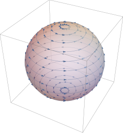
  Consider the sphere ${𝐒}^2$ in polar coordinates with the vector field $X={\partial }_{\varphi }$. The integral curves solve the equation (2.64), which are

  ${\displaystyle \frac{d\varphi }{dt}}=1\mathit{\hspace{1em}\hspace{1em} }\mathrm{and}\mathit{\hspace{1em}\hspace{1em} }{\displaystyle \frac{d\theta }{dt}}=0$

  This has the solution $\theta ={\theta }_0$ and $\varphi ={\varphi }_0+t$. The associated one-parameter diffeomorphism is ${\sigma }_t:(\theta ,\varphi )\to (\theta ,\varphi +t)$, and the flow lines are simply lines of constant latitude on the sphere and are shown in the left-hand figure.

• •

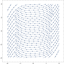
  Alternatively, consider the vector field on ${𝐑}^2$ with Cartesian components $X^{\mu }=(1,x^2)$. The equation for the integral curves is now

  ${\displaystyle \frac{dx}{dt}}=1\mathit{\hspace{1em}\hspace{1em} }\mathrm{and}\mathit{\hspace{1em}\hspace{1em} }{\displaystyle \frac{dy}{dt}}=x^2$

  which has the solution $x(t)=x_0+t$ and $y(t)=y_0+\frac{1}{3}{(x_0+t)}^3$. The associated flow lines are shown in the right-hand figure.

Next we ask: is it possible to differentiate a vector field? Specifically, suppose that we have a second vector field $Y$. How can we differentiate this in the direction of $X$ to get a new vector field? As we’ve seen, we can’t just write down $XY$ because this doesn’t define a new vector field.

To proceed, we should think more carefully about what differentiation means. For a function $f(x)$ on $𝐑$, we compare the values of the function at nearby points, and see what happens as those points approach each other

${\displaystyle \frac{df}{dx}}=\underset{t\to 0}{lim}{\displaystyle \frac{f(x+t)-f(x)}{t}}$

Similarly, to differentiate a vector field, we need to subtract the tangent vector $Y_p\in T_p(M)$ from the tangent vector at some nearby point $Y_q\in T_q(M)$, and then see what happens in the limit $q\to p$. But that’s problematic because, as we stressed above, the vector spaces $T_p(M)$ and $T_q(M)$ are different, and it makes no sense to subtract vectors in one from vectors in the other. To make progress, we’re going to have to find a way to do this. Fortunately, there is a way.

For example, if we have a function on $f:N\to 𝐑$, then we can construct a new function that we denote $({\phi }^{\ast }f):M\to 𝐑$,

$({\phi }^{\ast }f)(p)=f(\phi (p))$

Using the map in this way, to drag objects originally defined on $N$ onto $M$ is called the pull-back. If we introduce coordinates $x^{\mu }$ on $M$ and $y^{\alpha }$ on $N$, then the map $\phi (x)=y^{\alpha }(x)$, and we can write

$({\phi }^{\ast }f)(x)=f(y(x))$

Some objects more naturally go the other way. For example, given a vector field $Y$ on $M$, we can define a new vector field $({\phi }_{\ast }Y)$ on $N$. If we are given a function $f:N\to 𝐑$, then the vector field $({\phi }_{\ast }Y)$ on $N$ acts as

$({\phi }_{\ast }Y)(f)=Y({\phi }^{\ast }f)$

where I’ve been a little sloppy in the notation here since the left-hand side is a function on $N$ and the right-hand side a function on $M$. The equality above holds when evaluated at the appropriate points: $[({\phi }_{\ast }Y)(f)](\phi (p))=[Y({\phi }^{\ast }f)](p)$. Using the map to push objects on $M$ onto $N$ is called the push-forward.

If $Y=Y^{\mu }\partial /\partial x^{\mu }$ is the vector field on $M$, we can write the induced vector field on $N$ as

$({\phi }_{\ast }Y)(f)=Y^{\mu }{\displaystyle \frac{\partial f(y(x))}{\partial x^{\mu }}}=Y^{\mu }{\displaystyle \frac{\partial y^{\alpha }}{\partial x^{\mu }}}{\displaystyle \frac{\partial f(y)}{\partial y^{\alpha }}}$

Written in components, $({\phi }_{\ast }Y)={({\phi }_{\ast }Y)}^{\alpha }\partial /\partial y^{\alpha }$, we then have

${({\phi }_{\ast }Y)}^{\alpha }=Y^{\mu }{\displaystyle \frac{\partial y^{\alpha }}{\partial x^{\mu }}}$

(2.66)

Given the way that the indices are contracted, this is more or less the only thing we could write down.

We’ll see other examples of these induced maps later in the lectures. The push-forward is always denoted as ${\phi }_{\ast }$ and goes in the same way as the original map. The pull-back is always denoted as ${\phi }^{\ast }$ and goes in the opposite direction to the original map. Importantly, if our map $\phi :M\to N$ is a diffeomorphism, then we also have ${\phi }^{-1}:N\to M$, so we can transport any object from $M$ to $N$ and back again with impunity.

It will turn out that we can use these ideas to differentiate many different kinds of objects. As a warm-up, let’s first see how an analogous construction allows us to differentiate functions. Now the function

${ℒ}_{X}f=\underset{t\to 0}{lim}{\displaystyle \frac{f({\sigma }_t(x))-f(x)}{t}}={{\displaystyle \frac{df({\sigma }_t(x))}{dt}}|}_{t=0}={{\displaystyle \frac{\partial f}{\partial x^{\mu }}}{\displaystyle \frac{d{x}^{\mu }}{dt}}|}_{t=0}$

But, using (2.64), we know that $d{x}^{\mu }/dt=X^{\mu }$. We then have

${ℒ}_{X}f=X^{\mu }(x){\displaystyle \frac{\partial f}{\partial x^{\mu }}}=X(f)$

(2.67)

In other words, acting on functions with the Lie derivative ${ℒ}_X$ coincides with action of the vector field $X$.

Now let’s look at the action of ${ℒ}_X$ on a vector field $Y$. This is defined by

${ℒ}_{X}Y=\underset{t\to 0}{lim}{\displaystyle \frac{{({({\sigma }_{-t})}_{\ast }Y)}_p-Y_p}{t}}$

Note the minus sign in ${\sigma }_{-t}$. This reflects that fact that vector fields are pushed, rather than pulled. The map ${\sigma }_t$ takes us from the point $p$ to the point ${\sigma }_t(p)$. But to push a tangent vector $Y_{{\sigma }_t(p)}\in T_{{\sigma }_t(p)}(M)$ to a tangent vector in $T_p(M)$, where it can be compared to $Y_p$, we need to push with the inverse map ${({\sigma }_{-t})}_{\ast }$. This is shown Figure 20.

Let’s first calculate the action of ${ℒ}_X$ on a coordinate basis ${\partial }_{\mu }=\partial /\partial x^{\mu }$. We have

${ℒ}_X{\partial }_{\mu }=\underset{t\to 0}{lim}{\displaystyle \frac{{({\sigma }_{-t})}_{\ast }{\partial }_{\mu }-{\partial }_{\mu }}{t}}$

(2.68)

We have an expression for the push-forward of a tangent vector in (2.66), where the coordinates $y^{\alpha }$ on $N$ should now be replaced by the infinitesimal change of coordinates induced by the flow ${\sigma }_{-t}$ which, from (2.65) is $x^{\mu }(t)=x^{\mu }(0)-t{X}^{\mu }+\mathrm{\dots }$. Note the minus sign, which comes from the fact that we have to map back to where we came from as shown in Figure 20. We have, for small $t$,

${({\sigma }_{-t})}_{\ast }{\partial }_{\mu }=\left({\delta }_{\mu }^{\nu }-t{\displaystyle \frac{\partial X^{\nu }}{\partial x^{\mu }}}+\mathrm{\dots }\right){\partial }_{\nu }$

Acting on a coordinate basis, we then have

${ℒ}_X{\partial }_{\mu }=-{\displaystyle \frac{\partial X^{\nu }}{\partial x^{\mu }}}{\partial }_{\nu }$

(2.69)

To determine the action of ${ℒ}_X$ on a general vector field $Y$, we use the fact that the Lie derivative obeys the usual properties that we expect of a derivative, including linearity, ${ℒ}_X(Y_1+Y_2)={ℒ}_X{Y}_1+{ℒ}_X{Y}_2$ and Leibnizarity ${ℒ}_X(fY)=f{ℒ}_{X}Y+({ℒ}_{X}f)Y$ for any function $f$, both of which follow from the definition. The action on a general vector field $Y=Y^{\mu }(x)\partial /\partial x^{\mu }$ can then be written as

${ℒ}_X(Y^{\mu }{\partial }_{\mu })=({ℒ}_X{Y}^{\mu }){\partial }_{\mu }+Y^{\mu }({ℒ}_X{\partial }_{\mu })$

where we’ve simply viewed the components $Y^{\mu }(x)$ as $n$ functions. We can use (2.67) to determine ${ℒ}_X{Y}^{\mu }$ and we’ve computed ${ℒ}_X{\partial }_{\mu }$ in (2.69). We then have

${ℒ}_X(Y^{\mu }{\partial }_{\mu })=X^{\nu }{\displaystyle \frac{\partial Y^{\mu }}{\partial x^{\nu }}}{\partial }_{\mu }-Y^{\mu }{\displaystyle \frac{\partial X^{\nu }}{\partial x^{\mu }}}{\partial }_{\nu }$

But this is precisely the structure of the commutator. We learn that the Lie derivative acting on vector fields is given by

${ℒ}_{X}Y=[X,Y]$

A corollary of this is

${ℒ}_X{ℒ}_{Y}Z-{ℒ}_Y{ℒ}_{X}Z={ℒ}_{[X,Y]}Z$

(2.70)

which follows from the Jacobi identity for commutators.

The Lie derivative is just one of several derivatives that we will meet in this course. As we introduce new objects, we will learn how to act with ${ℒ}_X$ on them. But we will also see that we can endow different meanings to the idea of differentiation. In fact, the Lie derivative will take something of a back seat until Section 4.3 when we will see that it is what we need to understand symmetries.

We can also construct fields of cotangent vectors, by picking a member of $T_p^{\ast }(M)$ for each point $p$ in a smooth manner. Such a cotangent field is better known as a one-form; they map vector fields to real numbers. The set of all one-forms on $M$ is denoted ${\mathrm{\Lambda }}^1(M)$.

There is a particularly simple way to construct a one-form. Take a function $f\in C^{\mathrm{\infty }}(M)$ and define $df\in {\mathrm{\Lambda }}^1(M)$ by

$df(X)=X(f)$

(2.71)

We can use this method to build a basis for ${\mathrm{\Lambda }}^1(M)$. If we introduce coordinates $x^{\mu }$ on $M$ with the corresponding coordinate basis $e_{\mu }=\partial /\partial x^{\mu }$ of vector fields, which we often write in shorthand as $\partial /\partial x^{\mu }\equiv {\partial }_{\mu }$. We then we simply take the functions $f=x^{\mu }$ which, from (2.71), gives

$d{x}^{\mu }({\partial }_{\nu })={\partial }_{\nu }(x^{\mu })={\delta }_{\nu }^{\mu }$

This means that $f^{\mu }=d{x}^{\mu }$ provides a basis for ${\mathrm{\Lambda }}^1(M)$, dual to the coordinate basis $\partial /{\partial }_{\mu }$. In general, an arbitrary one-form $\omega \in {\mathrm{\Lambda }}^1(M)$ can then be expanded as

$\omega ={\omega }_{\mu }d{x}^{\mu }$

In such a basis the one-form $df$ takes the form

$df={\displaystyle \frac{\partial f}{\partial x^{\mu }}}d{x}^{\mu }$

(2.72)

To see this, we simply need to evaluate

$df(X)={\displaystyle \frac{\partial f}{\partial x^{\mu }}}d{x}^{\mu }(X^{\nu }{\partial }_{\nu })=X^{\mu }{\displaystyle \frac{\partial f}{\partial x^{\mu }}}=X(f)$

which agrees with the expected answer (2.71).

As with vector fields, we can look at what happens if we change coordinates. Given two different charts, $\varphi =(x^1,\mathrm{\dots },x^n)$ and $\tilde{\varphi }=({\tilde{x}}^1,\mathrm{\dots },{\tilde{x}}^n)$, we know that the basis for vector fields changes as (2.60),

${\displaystyle \frac{\partial }{\partial {\tilde{x}}^{\mu }}}={\displaystyle \frac{\partial x^{\nu }}{\partial {\tilde{x}}^{\mu }}}{\displaystyle \frac{\partial }{\partial x^{\nu }}}$

We should take the basis of one-forms to transform in the inverse manner,

$d{\tilde{x}}^{\mu }={\displaystyle \frac{\partial {\tilde{x}}^{\mu }}{\partial x^{\nu }}}d{x}^{\nu }$

(2.73)

This then ensures that

$d{\tilde{x}}^{\mu }\left({\displaystyle \frac{\partial }{\partial {\tilde{x}}^{\nu }}}\right)={\displaystyle \frac{\partial {\tilde{x}}^{\mu }}{\partial x^{\rho }}}d{x}^{\rho }\left({\displaystyle \frac{\partial x^{\sigma }}{\partial {\tilde{x}}^{\nu }}}{\displaystyle \frac{\partial }{\partial x^{\sigma }}}\right)={\displaystyle \frac{\partial {\tilde{x}}^{\mu }}{\partial x^{\rho }}}{\displaystyle \frac{\partial x^{\sigma }}{\partial {\tilde{x}}^{\nu }}}d{x}^{\rho }\left({\displaystyle \frac{\partial }{\partial x^{\sigma }}}\right)={\displaystyle \frac{\partial {\tilde{x}}^{\mu }}{\partial x^{\rho }}}{\displaystyle \frac{\partial x^{\sigma }}{\partial {\tilde{x}}^{\nu }}}{\delta }_{\sigma }^{\rho }$

But this is just the multiplication of a matrix and its inverse,

${\displaystyle \frac{\partial {\tilde{x}}^{\mu }}{\partial x^{\rho }}}{\displaystyle \frac{\partial x^{\rho }}{\partial {\tilde{x}}^{\nu }}}={\delta }_{\nu }^{\mu }$

So we find that

$d{\tilde{x}}^{\mu }\left({\displaystyle \frac{\partial }{\partial {\tilde{x}}^{\nu }}}\right)={\delta }_{\nu }^{\mu }$

as it should. We can then expand a one-form $\omega$ in either of these two bases,

$\omega ={\omega }_{\mu }d{x}^{\mu }={\tilde{\omega }}_{\mu }d{\tilde{x}}^{\mu }\mathit{\hspace{1em}\hspace{1em} }\mathrm{with}\mathit{\hspace{1em}\hspace{1em} }{\tilde{\omega }}_{\mu }={\displaystyle \frac{\partial x^{\nu }}{\partial {\tilde{x}}^{\mu }}}{\omega }_{\nu }$

(2.74)

In the annoying terminology that I can never remember, components of vectors that transform this way are said to be covariant. Note that, as with vector fields, the placement of the indices means that (2.73) and (2.74) are pretty much the only things that you can write down that make sense.