10.2  The EM approximations

Ith = Ab(Z)   ó õ T   C(T, Ne)  Ne NH  dh dT dT

(29)

Many authors (e.g. Pottasch 1963; Jordan and Wilson 1971) approximate the above expression by removing an averaged value of C(T) from the integral:

Ith = Ab(Z)   < C(T) >   ó õ h   Ne NH dh

(30)

A suitably defined volume line emission measure EM_L can therefore be defined, for each observed line of intensity I_ob:

EML º  Iob Ab(Z)   < C(T) >      [cm-5]

(31)

The relative abundances of the elements are derived in order to have all the line emission measures of the various ions lie along a common smooth curve.

10.2.1  A different approximation. The Widing and Feldman method

A different approach was proposed by Widing and Feldman (1989):

extract from the integral an averaged value of the DEM of the line, that here is termed the line DEM DEM_L:

DEML º < Ne NH  dh dT >     [cm-5 K-1]

(32)

such that for each line of observed intensity I_ob:

DEML º   Iob Ab(Z)   ó õ T   C(T) dT

(33)

A plot of the A_b(Z)   DEM_L = I_ob / ò_T  C(T) dT values displayed at the temperatures T_max is used to deduce relative element abundances, adjusting them in order to have a continuous sequence of the A_b(Z)   DEM_L values.

10.2.2  Various problems

Only when the two lines have similar C(T) and the DEM distribution is relatively flat would one expect that the DEM factors out from the integrals:

ó õ T    C1(T, Ne)  DEM (T)  dT ó õ T    C2(T, Ne)  DEM (T)  dT = ó õ T    C1(T, Ne)  dT ó õ T    C2(T, Ne)  dT

(34)

If the above equality holds, then it is possible to deduce the relative abundances directly from the observed intensities and the contribution functions, because:

Ab(X1) Ab(X2) = I1 ·  ó õ T    C2(T, Ne)  dT I2 ·  ó õ T    C2(T, Ne)  dT =  DEML(X2) DEML(X1)

(35)

i.e. the DEM method and the DEM_L method are equivalent.

However, this is not always the case.

10.2.3  AR abundances

Figure 35: [from Del Zanna (2003)] SOHO CDS and TRACE images of the base of an active region loop system.

Figure 36: Left: Widing & Feldman (1993) method, FIP=14 Right: EM loci results, FIP=3.7, 4 times lower !

Many other effects can significantly affect results. For example:

- Blending

- Density effects

- The uncertainty on the ionisation fractions

10.2.4  Coronal hole plumes

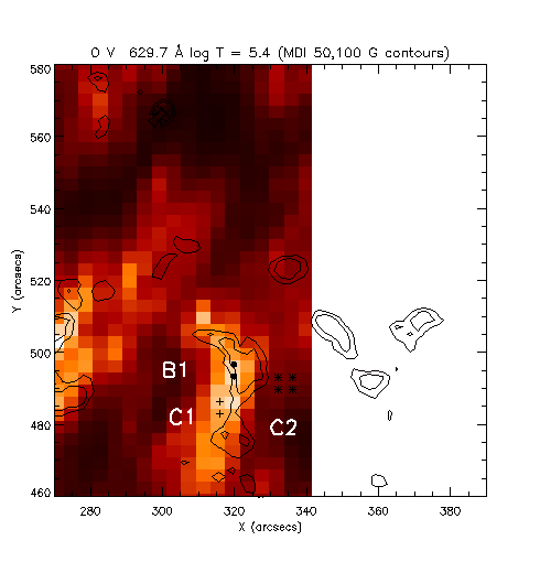
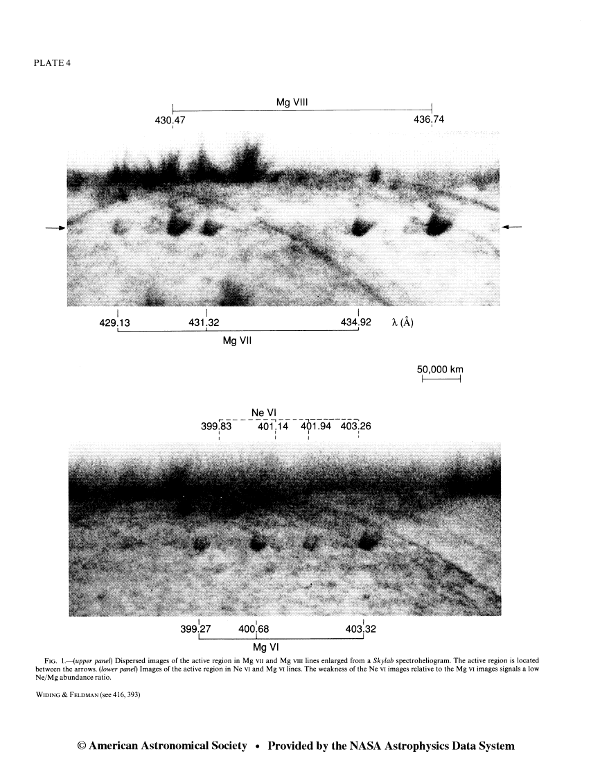
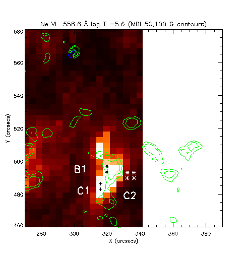
One of the highest FIP effects was measured by Widing & Feldman (1992) on the bright coronal hole plume observed by Skylab. A DEM analysis was performed on the calibrated data tabulated in Widing & Feldman, using photospheric abundances as a starting point.

Figure 37: [from Del Zanna et al. 2003] Left: DEM_L values from Widing & Feldman (1992), and FIP=10. Right: The DEM_L values for the Skylab plume, and photospheric abundances. The Ne and Mg values indicate the need to modify the adopted Ne/Mg photospheric abundance ratio, in order to obtain a smooth distribution of DEM_L values. The DEM(T) derived from the same data is plotted for comparison (dashed line).

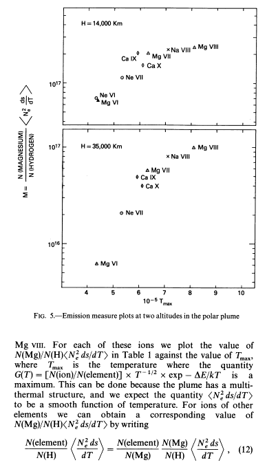
Fig. 37 shows the DEM_L values for the Skylab plume. Following the DEM_L method, the points are displayed at the temperatures T_max, defined as the temperature where C(T) has a maximum. First, we note that the use of T_max is misleading since, this is quite different from the temperature at which most of the emission occurs.

It is often more informative to use an ``effective temperature" T_eff, defined as

log   Teff = ó õ C(T)  DEM(T) log   T  dT / ( ó õ C(T)  DEM(T)  dT)

Fig. 37 clearly shows that, in order to align the DEM_L points on a smooth curve, it is necessary to modify the adopted Mg/Ne relative abundances by a large factor, consistent with the FIP effect found by Widing and Feldman.

Figure 38: [from Del Zanna et al. 2003] The I_ob / (A_b * C(T)) curves for the Skylab plume, assuming photospheric abundances. The data indicate an isothermal distribution at log T=5.9 and are consistent with no FIP effect present. The emission measure EM(0.1) values calculated with the DEM of Fig. 37 and a Dlog T=0.1 are also shown (filled circles).

A DEM analysis has been performed on the dataset, and the result displayed as a dashed line in Fig. 37. It is clear that there is a large difference between the DEM_L points and the DEM values.

The I_ob / (A_b * C(T)) curves for the plume, calculated with photospheric abundances, are displayed in Fig. 38. They clearly show that the plasma is nearly isothermal, since all the curves are crossing at one point (with the exception of the Ne VII 465.2 Å resonance line, which clearly departs from this behaviour and requires further investigation). The figure also shows that the observed Mg VI and Ne VI intensities are consistent with photospheric abundances.

---

File translated from T_EX by T_TH, version 3.08.
On 13 Sep 2004, 23:34.