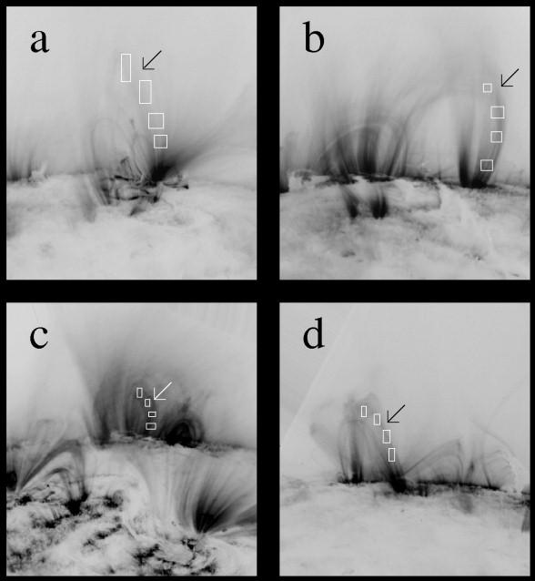
1.2 The TRACE loops
Figure 8: [From Lenz et al., 1999]
Images in the 171 Å filter of the loops selected for this study
(indicated by arrows): (a) 1998 July 4, (b) 1998 July 26, (c) 1998
August 18,
(d) 1998 August 20. Images have been rotated so that the limb is
roughly horizontal. The field of view of each image is 56×54 (roughly
680×650 pixels).
Figure 9: [From Lenz et al., 1999]
(a) Temperature and (b) emission measure as functions of fractional distance along the loop for loop a (plus signs), loop b (diamonds),
loop c (triangles), loop d (squares),
and model loop 3 with T=1.34 MK and uniform line-of-sight depth D=10 cm (connected asterisks).
Also shown in (b) are model loop 1: an isothermal (T=1.34 MK),
hydrostatic loop with a uniform line-of-sight depth (dashed line); and model
loop 2: the same as model loop 1, but with a line-of-sight depth that
increases along the loop by a factor of 4 (dot-dashed line).
The errors on the observations are comparable to or less than the size
of the plot symbols.
Figure 3: [From Aschwanden et al., 2000]
Figure 4: [From Aschwanden et al., 2000]
Normalized temperature profiles Te(s)/Te(L) (top) and density profiles
ne(s) (bottom) of the steady state model
(RTV/Serio) are shown (thick lines) in comparison with the actual
best-fit models to the observed TRACE data (thin
lines, numbered from 1 to 41 for individual loops). The theoretical
density profiles (RTV/Serio) are calculated for loop
lengths of L = 10, 50, 100, 150, 200 Mm. Note that the observed
densities agree only for the shortest loops (L < 10 Mm),
while they are about an order of magnitude higher for larger loops
(L simeq 50-250 Mm). The observed temperature
profiles are always flatter than the theoretically predicted ones.
Figure 5: Top: [From Aschwanden et al., 2000] 26 July 1998
26 July 1998 - Loops 28 (same as in Lenz et al. 1999),
24 as in Aschwanden et al., 2000.
Figure 6:
Figure 7: