Many problems in imaging can be formulated as problems of statistical inference. That are problems the of type: Find a true parameter given observed data that is somehow related to the parameter. In image denoising, for instance, we aim to identify the noise-free image (parameter) given a noisy version of this image (data). In X-ray computed tomography, on the other hand, we are given a sinogram from a CT scanner (data) and aim to reconstruct the absorption coefficient (parameter) of the scanned body.
Statistically speaking, such problems are usually solved with a maximum likelihood or maximum-a-posteriori approach. This gives a point estimator of the image, which we might call the “reconstructed image”. Especially - but not exclusively - in the presence of observational noise, an obvious question is: How certain can we be about the reconstructed images? Does it actually show the underlying truth? Which part of the reconstruction can we be certain about? Where do we have to be careful?
We aim to answer these questions by employing a Bayesian approach to image reconstruction. Bayesian approach means, we represent the reconstructed image as a random variable. Rather than actual randomness, this random variable represents our uncertainty about the image before seeing the data. The distribution of this random variable is called “prior distribution”. Using Bayes’ formula and our observed data, we can “update” this prior distribution and obtain the conditional distribution of the image given the observed data. This conditional distribution is called “posterior distribution”. It represents our uncertainty in the image after seeing the data.
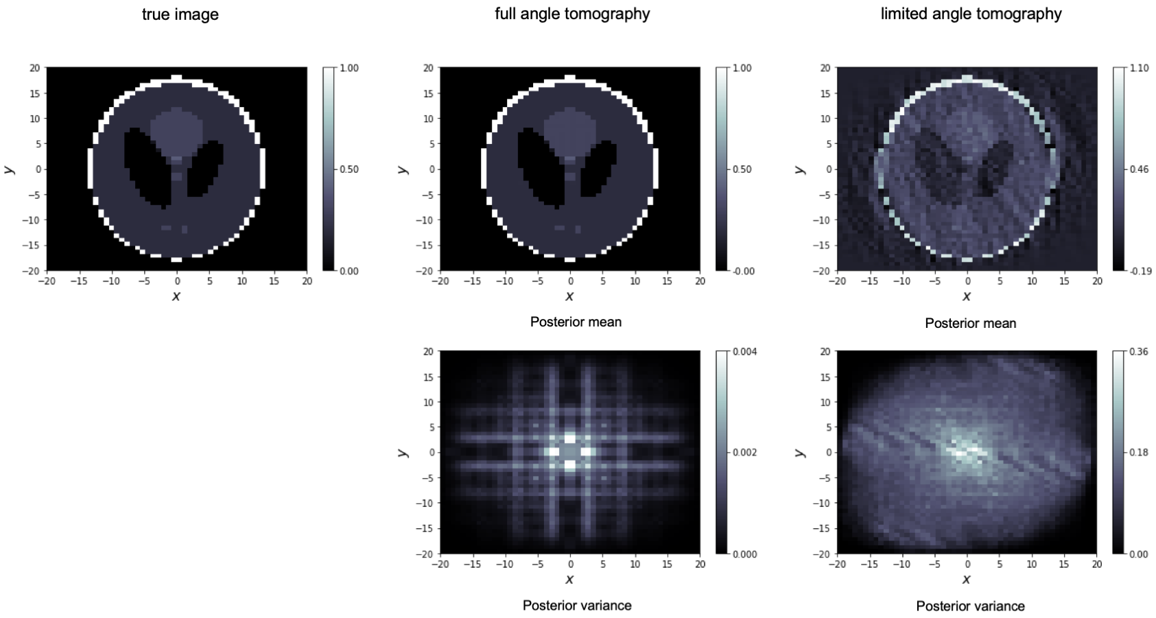
We give an example above. Here, we perform a Bayesian CT reconstruction with a phantom data set, which we show to the very left. The prior is Gaussian white noise and we assume that the sinogram was polluted by additive scaled Gaussian white noise. We have computed the posterior mean and the pixelwise posterior variance in the case of full angle tomography (centre column) and the case of limited angle tomography (right column). Not only the posterior mean estimate is worse in the limited angle case, also the variance is orders of magnitude larger. This precisely reflects our intuition: in limited angle tomography, we have seen fewer data points and, thus, are more uncertain.