9.2  Density and temperature diagnostics from line intensities

The theoretical intensity ratios from individual ion species provide a measurement of electron density which is independent of any assumptions about the volume of the emitting region.

DENS_PLOTTER and TEMP_PLOTTER are high-level widgets for the analysis of density- and temperature-sensitive ratios of lines from the same ion. They allow inclusion of proton rates and photoexcitation. The calling sequence is simple:

 IDL > dens_plotter,'o_5'

to study O V.

 IDL > temp_plotter,'c_4'

to study C IV.

9.2.1  Density

Figure 40: The density-sensitive Si IX ratio and its variation with temperature.

1. Temperature effects should be taken into account.

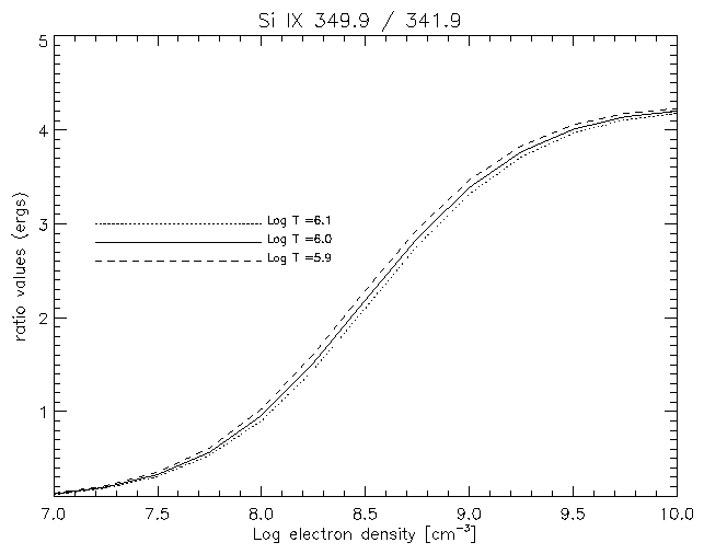
   Figure 41 shows the density-sensitive Si IX ratio calculated at three temperatures (T=10⁶ K is the temperature of maximum ionization fraction for Si IX), showing that these temperature variations do not appreciably affect the ratio.

2. Photoexcitation can be important for some ions.

   The radiation that comes from the solar photosphere can excite transitions between levels in the ground configuration of ions in the corona, mainly affecting the level balance calculations for low densities (N_e £ 10⁸ cm^-3).

   The effect is stronger close to the photosphere, and tends to die out with height because of the decrease of the photospheric radiation field with distance. This decrease can be accounted for by estimating a geometric dilution factor that is a function of height above the photosphere. Si IX should be affected more than other ions.

3. Most of the observed diagnostic lines are very weak, which makes the data analysis difficult.
4. For some ions, the atomic data are yet not reliable. For example, do not use Fe XII !!.

5. Many diagnostic ratios are affected by blending which varies depending on the type of source observed, and which is particularly strong at the moderate resolution of CDS.
6. Only ions that have peak emissivity at the temperatures where the source emits can be expected to give meaningful results.
7. The densites that are obtained do depend on the chosen instrument calibration. The various calibrations do agree within 30% on average, but larger departures are present in some cases (see Del Zanna et al. 2001).
8. Many density estimates found in the literature are not correct, for a variety of reasons.

Figure 41: Some useful density-sensitive line ratios observed by CDS.

Table 2: Density sensitive line ratios observed by CDS, ordered by the temperature of maximum of the contribution functions shown in column 4, calculated with the ionization equilibrium calculations of Arnaud and Rothenflug (1985). The ranges for which the ratios can be used are shown in column 5. The numbers in parentheses indicate the number of transitions that compose the self-blends. The lines indicated with a (!) have problems in either their observation or in the atomic physics. The lines indicated with a (*) are the best selection within a wider choice. The detectors in parentheses indicate that the lines are also visible in second order. N means NIS, and G means GIS;

Ion	Ratio (Å)	Detector	log Tmax	log Ne
Si IX (*)	349.9 (3) / 341.949	N 1 (G 4)	6.02	7.5 - 9.5
Si IX	345.100 / 341.949	N 1 (G 4)	6.02	7.5 - 9.5
Si IX	349.9 (3) / 345.100	N 1 (G 4)	6.02	7.5 - 9.5
Si X	356.0 (2) / 347.402	N 1 (G 4)	6.12	8.0 - 10.0
Fe XII	338.278 (!) / 364.467	N 1 (G 4)	6.16	7.0 - 12.0
Fe XIII	321.4 / 320.80	N 1	6.21	8 - 10
Fe XIII	318.12 / 320.80	N 1	6.21	8 - 10
Fe XIII	359.6 (2) (!) / 348.18	N 1 (G 4)	6.21	8 - 10
Fe XIII (*)	320.8 (bl) / 348.18	N 1	6.21	8 - 10
Fe XIII (*)	203.8 (2) / 202.044	G 1	6.21	8.5 - 10.5
Fe XIV	353.83 (!) / 334.17	N 1 (G 4)	6.25	9.0 - 11.0

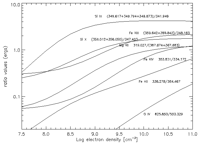
Table 2 presents a list of useful density-sensitive line ratios available within the CDS channels. Only the principal usable ratios are listed, involving pairs of lines seen by the same spectrometer and detector.

The lines indicated with a (!) have problems in either their observation or in the atomic physics. This is based on experience gained in analysing different source regions (e.g. on-disc, off-limb, coronal holes, quiet sun, active regions) with the different detectors, and on the best possible line identification, with DEM analysis of the various regions.

Further examples and details are given in my thesis.

9.2.2  A better (global) approach

Figure 42: Emissivities calculated with CHIANTI

It is common in the literature to use only a few well-behaved line ratios, without considering all the observed lines. A different approach, preferable when more than two lines from an ion are observed, is to plot the values of

Fji =   I(lij) Ne h nij  Nj(Ne)   Aji

(19)

as a function of electron density, calculated at a fixed temperature. All the curves should cross at one point, if the plasma is isodensity. The F_ji curves should be calculated at the effective temperature, i.e. at the temperature where the bulk of the ion emission is (see Del Zanna et al. 2002).

Figure 43: [From Del Zanna et al. 2003] The F_ji curves from a whole-Sun grazing incidence spectrum. Note that the intensities of the 257.26 and 182.3 have been rescaled taking into account the known blends.

9.2.3  The electron temperature evaluation. The isothermal case

Once the isothermal assumption is made, it is straightforward to deduce from a line ratio a temperature T_*, since the intensity ratio I₁/I₂ is directly equal to the ratio of the contribution functions:

I1 I2 =  C1(T*, Ne) C2(T*, Ne)

(20)

Any ratios of lines of ions of close ionization stage can be used for this purpose, as long as the lines are not density-sensitive, otherwise the derived temperature T_* becomes density-dependent.

Different line ratios are expected to give different temperatures, if the plasma distribution is not isothermal.

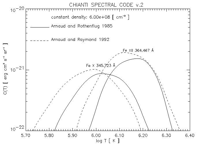
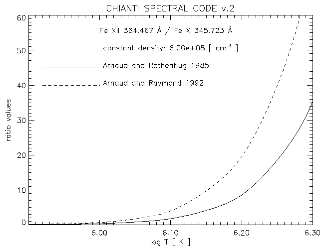
Aside from the cited possible errors due to density and element abundance uncertainties, which can easily be avoided by careful choice of lines, there is one substantial source of error that surprisingly is normally neglected in the literature. This is the validity of the adopted ionization equilibrium.

The use of different ionization equilibrium calculations can produce significantly different results as shown in Figure 45.

Figure 44: Contribution functions of two iron lines and their ratio, for different ionization equilibria. Note how the ratio is different.

A more direct way to deduce electron temperatures is to use the ratio of two lines of the same ion. Examples are given in my thesis.