2 Classical Gases 4 Classical Thermodynamics

3 Quantum Gases

In this section we will discuss situations where quantum effects are important. We’ll still restrict attention to gases — meaning a bunch of particles moving around and barely interacting — but one of the first things we’ll see is how versatile the idea of a gas can be in the quantum world. We’ll use it to understand not just the traditional gases that we met in the previous section but also light and, ironically, certain properties of solids. In the latter part of this section, we will look at what happens to gases at low temperatures where their behaviour is dominated by quantum statistics.

3.1 Density of States

We start by introducing the important concept of the density of states. To illustrate this, we’ll return once again to the ideal gas trapped in a box with sides of length $L$ and volume $V=L^{3}$ . Viewed quantum mechanically, each particle is described by a wavefunction. We’ll impose periodic boundary conditions on this wavefunction (although none of the physics that we’ll discuss in this course will be sensitive to the choice of boundary condition). If there are no interactions between particles, the energy eigenstates are simply plane waves,

\displaystyle\psi=\frac{1}{\sqrt{V}}\,e^{i\vec{k}\cdot\vec{x}}

Boundary conditions require that the wavevector $\vec{k}=(k_{1},k_{2},k_{3})$ is quantized as

\displaystyle k_{i}=\frac{2\pi n_{i}}{L}\ \ {\rm with}\ \ n_{i}\in{\bf Z}

and the energy of the particle is

\displaystyle E_{\vec{n}}=\frac{\hbar^{2}{k}{}^{2}}{2m}=\frac{4\pi^{2}\hbar^{2% }}{2mL^{2}}\,(n_{1}^{2}+n_{2}^{2}+n_{3}^{2})

with $k=|\vec{k}|$ . The quantum mechanical single particle partition function (1.21) is given by the sum over all energy eigenstates,

\displaystyle Z_{1}=\sum_{\vec{n}}e^{-\beta E_{\vec{n}}}

The question is: how do we do the sum? The simplest way is to approximate it by an integral. Recall from the previous section that the thermal wavelength of the particle is defined to be

\displaystyle\lambda=\sqrt{\frac{2\pi\hbar^{2}}{mk_{B}T}}

The exponents that appear in the sum are all of the form $\sim\lambda^{2}n^{2}/L^{2}$ , up to some constant factors. For any macroscopic size box, $\lambda\ll L$ (a serious understatement! Actually $\lambda\ll\!\!\ll L$ ) which ensures that there are many states with $E_{\vec{n}}\leq k_{B}T$ all of which contribute to the sum. (There will be an exception to this at very low temperatures which will be the focus of Section 3.5.3). We therefore lose very little by approximating the sum by an integral. We can write the measure of this integral as

\displaystyle\sum_{\vec{n}}\ \approx\ \int d^{3}n\ =\ \frac{V}{(2\pi)^{3}}\int d% ^{3}k=\ \frac{4\pi V}{(2\pi)^{3}}\int_{0}^{\infty}dk\ k^{2}

where, in the last equality, we have integrated over the angular directions to get $4\pi$ , the area of the 2-sphere, leaving an integration over the magnitude $k=|\vec{k}|$ and the Jacobian factor $k^{2}$ . For future applications, it will prove more useful to change integration variables at this stage. We work instead with the energy,

\displaystyle E=\frac{\hbar^{2}{k}^{2}}{2m}\ \ \ \Rightarrow\ \ \ dE=\frac{% \hbar^{2}{k}}{m}\,dk

We can now write out integral as

\displaystyle\frac{4\pi V}{(2\pi)^{3}}\int dk\ k^{2}\ =\ \frac{V}{2\pi^{2}}% \int dE\ \sqrt{\frac{2mE}{\hbar^{2}}}\frac{m}{\hbar^{2}}\ \equiv\ \int dE\ g(E)

(3.90)

where

\displaystyle g(E)=\frac{V}{4\pi^{2}}\left(\frac{2m}{\hbar^{2}}\right)^{3/2}E^% {1/2}

(3.91)

is the density of states: $g(E)dE$ counts the number of states with energy between $E$ and $E+dE$ . Notice that we haven’t actually done the integral over $E$ in (3.90); instead this is to be viewed as a measure which we can integrate over any function $f(E)$ of our choosing.

There is nothing particularly quantum mechanical about the density of states. Indeed, in the derivation above we have replaced the quantum sum with an integral over momenta which actually looks rather classical. Nonetheless, as we encounter more and more different types of gases, we’ll see that the density of states appears in all the calculations and it is a useful quantity to have at our disposal.

3.1.1 Relativistic Systems

Relativistic particles moving in $d=3+1$ spacetime dimensions have kinetic energy

\displaystyle E=\sqrt{\hbar^{2}k^{2}c^{2}+m^{2}c^{4}}

(3.92)

Repeating the steps above, we find the density of states is given by

\displaystyle g(E)=\frac{VE}{2\pi^{2}\hbar^{3}c^{3}}\,\sqrt{E^{2}-m^{2}c^{4}}

(3.93)

In particular, for massless particles, the density of states is

\displaystyle g(E)

\displaystyle=

\displaystyle\frac{VE^{2}}{2\pi^{2}\hbar^{3}c^{3}}

(3.94)

3.2 Photons: Blackbody Radiation

“It was an act of desperation. For six years I had struggled with the blackbody theory. I knew the problem was fundamental and I knew the answer. I had to find a theoretical explanation at any cost, except for the inviolability of the two laws of thermodynamics”

Max Planck

We now turn to our first truly quantum gas: light. We will consider a gas of photons — the quanta of the electromagnetic field — and determine a number of its properties, including the distribution of wavelengths. Or, in other words, its colour.

Below we will describe the colour of light at a fixed temperature. But this also applies (with a caveat) to the colour of any object at the same temperature. The argument for this is as follows: consider bathing the object inside the gas of photons. In equilibrium, the object sits at the same temperature as the photons, emitting as many photons as it absorbs. The colour of the object will therefore mimic that of the surrounding light.

For a topic that’s all about colour, a gas of photons is usually given a rather bland name — blackbody radiation. The reason for this is that any real object will exhibit absorption and emission lines due to its particular atomic make-up (this is the caveat mentioned above). We’re not interested in these details; we only wish to compute the spectrum of photons that a body emits because it’s hot. For this reason, one sometimes talks about an idealised body that absorbs photons of any wavelength and reflects none. At zero temperature, such an object would appear black: this is the blackbody of the title. We would like to understand its colour as we turn up the heat.

To begin, we need some facts about photons. The energy of a photon is determined by its wavelength $\lambda$ or, equivalently, by its frequency $\omega=2\pi c/\lambda$ to be

\displaystyle E=\hbar\omega

This is a special case of the relativistic energy formula (3.92) for massless particles, $m=0$ . The frequency is related to the (magnitude of the) wavevector by $\omega=kc$ .

Photons have two polarization states (one for each dimension transverse to the direction of propagation). To account for this, the density of states (3.94) should be multiplied by a factor of two. The number of states available to a single photon with energy between $E$ and $E+dE$ is therefore

\displaystyle g(E)dE=\frac{VE^{2}}{\pi^{2}\hbar^{3}c^{3}}dE

Equivalently, the number of states available to a single photon with frequency between $\omega$ and $\omega+d\omega$ is

\displaystyle g(E)dE=g(\omega)d\omega=\frac{V\omega^{2}}{\pi^{2}c^{3}}d\omega

(3.95)

where we’ve indulged in a slight abuse of notation since $g(\omega)$ is not the same function as $g(E)$ but is instead defined by the equation above. It is also worth pointing out an easy mistake to make when performing these kinds of manipulations with densities of states: you need to remember to rescale the interval $d E$ to $d\omega$ . This is most simply achieved by writing $g(E)dE=g(\omega)d\omega$ as we have above. If you miss this then you’ll get $g(\omega)$ wrong by a factor of $\hbar$ .

The final fact that we need is important: photons are not conserved. If you put six atoms in a box then they will still be there when you come back a month later. This isn’t true for photons. There’s no reason that the walls of the box can’t absorb one photon and then emit two. The number of photons in the world is not fixed. To demonstrate this, you simply need to turn off the light.

Because photon number is not conserved, we’re unable to define a chemical potential for photons. Indeed, even in the canonical ensemble we must already sum over states with different numbers of photons because these are all “accessible states”. (It is sometimes stated that we should work in the grand canonical ensemble at $\mu=0$ which is basically the same thing). This means that we should consider states with any number $N$ of photons.

We’ll start by looking at photons with a definite frequency $\omega$ . A state with $N$ such photons has energy $E=N\hbar\omega$ . Summing over all $N$ gives us the partition function for photons at fixed frequency,

\displaystyle Z_{\omega}=1+e^{-\beta\hbar\omega}+e^{-2\beta\hbar\omega}+\ldots% =\frac{1}{1-e^{-\beta\hbar\omega}}

(3.96)

Figure 14: The Planck Distribution function (Source: E. Schubert, Light Emitting Diodes).

We now need to sum over all possible frequencies. As we’ve seen a number of times, independent partition functions multiply, which means that the $\log$ s add. We only need to know how many photon states there are with some frequency $\omega$ . But this is what the density of states (3.95) tells us. We have

\displaystyle\log Z=\int_{0}^{\infty}d\omega\ g(w)\,\log Z_{\omega}=-\frac{V}{% \pi^{2}c^{3}}\int_{0}^{\infty}d\omega\ \omega^{2}\log\left(1-e^{-\beta\hbar% \omega}\right)

(3.97)

3.2.1 Planck Distribution

From the partition function (3.97) we can calculate all interesting quantities for a gas of light. For example, the energy density stored in the photon gas is

\displaystyle E=-\frac{\partial}{\partial{\beta}}\log Z=\frac{V\hbar}{\pi^{2}c% ^{3}}\int_{0}^{\infty}d\omega\ \frac{\omega^{3}}{e^{\beta\hbar\omega}-1}

(3.98)

However, before we do the integral over frequency, there’s some important information contained in the integrand itself: it tells us the amount of energy carried by photons with frequency between $\omega$ and $\omega+d\omega$

\displaystyle E(\omega)d\omega=\frac{V\hbar}{\pi^{2}c^{3}}\frac{\omega^{3}}{e^% {\beta\hbar\omega}-1}d\omega

(3.99)

This is the Planck distribution. It is plotted above for various temperatures. As you can see from the graph, for hot gases the maximum in the distribution occurs at a lower wavelength or, equivalently, at a higher frequency. We can easily determine where this maximum occurs by finding the solution to $dE(\omega)/d\omega=0$ . It is

\displaystyle\omega_{\rm max}=\zeta\frac{k_{B}T}{\hbar}

where $\zeta\approx 2.822$ solves $3-\zeta=3e^{-\zeta}$ . The equation above is often called Wien’s displacement law. Roughly speaking, it tells you the colour of a hot object.

To compute the total energy in the gas of photons, we need to do the integration in (3.98). To highlight how the total energy depends on temperature, it is useful to perform the rescaling $x=\beta\hbar\omega$ , to get

\displaystyle E=\frac{V}{\pi^{2}c^{3}}\frac{(k_{B}T)^{4}}{\hbar^{3}}\int_{0}^{% \infty}\frac{x^{3}dx}{e^{x}-1}

The integral $I=\int dx\,x^{3}/(e^{x}-1)$ is tricky but doable. It turns out to be $I=\pi^{4}/15$ . (We will effectively prove this fact later in the course when we consider a more general class of integrals (3.116) which can be manipulated into the sum (3.117). The net result of this is to express the integral $I$ above in terms of the Gamma function and the Riemann zeta function: $I=\Gamma(4)\zeta(4)=\pi^{4}/15$ ). We learn that the energy density ${\cal E}=E/V$ in a gas of photons scales is proportional to $T^{4}$ ,

\displaystyle{\cal E}=\frac{\pi^{2}k_{B}^{4}}{15\hbar^{3}c^{3}}\,T^{4}

Stefan-Boltzmann Law

The expression for the energy density above is closely related to the Stefan-Boltzmann law which describes the energy emitted by an object at temperature $T$ . That energy flux is defined as the rate of transfer of energy from the surface per unit area. It is given by

\displaystyle\mbox{Energy Flux}=\frac{{\cal E}c}{4}\equiv\sigma T^{4}

(3.100)

where

\displaystyle\sigma=\frac{\pi^{2}k_{B}^{4}}{60\hbar^{3}c^{2}}=5.67\times 10^{-% 8}\ Js^{-1}m^{-2}K^{-4}

is the Stefan constant.

The factor of the speed of light in the middle equation of (3.100) appears because the flux is the rate of transfer of energy. The factor of $1/4$ comes because we’re not considering the flux emitted by a point source, but rather by an actual object whose size is bigger than the wavelength of individual photons. This means that the photon are only emitted in one direction: away from the object, not into it. Moreover, we only care about the velocity perpendicular to the object, which is $(c\cos\theta)$ where $\theta$ is the angle the photon makes with the normal. This means that rather than filling out a sphere of area $4\pi$ surrounding the object, the actual flux of photons from any point on the object’s surface is given by

\displaystyle\frac{1}{4\pi}\int_{0}^{2\pi}d\phi\int_{0}^{\pi/2}d\theta\,\sin% \theta\ (c\cos\theta)=\frac{c}{4}

Radiation Pressure and Other Stuff

All other quantities of interest can be computed from the free energy,

	$\displaystyle F$	$\displaystyle=$	$\displaystyle-k_{B}T\log Z$
		$\displaystyle=$	$\displaystyle\frac{Vk_{B}T}{\pi^{2}c^{3}}\int_{o}^{\infty}d\omega\ \omega^{2}% \log\left(1-e^{-\beta\hbar\omega}\right)$

We can remove the logarithm through an integration by parts to get,

$\displaystyle F$	$\displaystyle=$	$\displaystyle-\frac{V\hbar}{3\pi^{2}c^{3}}\int_{0}^{\infty}d\omega\ \frac{% \omega^{3}e^{-\beta\hbar\omega}}{1-e^{-\beta\hbar\omega}}$
	$\displaystyle=$	$\displaystyle-\frac{V\hbar}{3\pi^{2}c^{3}}\frac{1}{\beta^{4}\hbar^{4}}\int_{0}% ^{\infty}dx\ \frac{x^{3}}{e^{x}-1}$
	$\displaystyle=$	$\displaystyle-\frac{V\pi^{2}}{45\hbar^{3}c^{3}}\,(k_{B}T)^{4}$

From this we can compute the pressure due to electromagnetic radiation,

\displaystyle p=-\left.\frac{\partial{F}}{\partial{V}}\right|_{T}=\frac{E}{3V}% =\frac{4\sigma}{3c}T^{4}

This is the equation of state for a gas of photons. The middle equation tells us that the pressure of photons is one third of the energy density — a fact which will be important in the Cosmology course.

We can also calculate the entropy $S$ and heat capacity $C_{V}$ . They are both most conveniently expressed in terms of the Stefan constant which hides most of the annoying factors,

\displaystyle S=-\left.\frac{\partial{F}}{\partial{T}}\right|_{V}=\frac{16V% \sigma}{3c}T^{3}\ \ \ \ ,\ \ \ \ C_{V}=\left.\frac{\partial{E}}{\partial{T}}% \right|_{V}=\frac{16V\sigma}{c}T^{3}

3.2.2 The Cosmic Microwave Background Radiation

The cosmic microwave background, or CMB, is the afterglow of the big bang, a uniform light that fills the Universe. The intensity of this light was measured accurately by the FIRAS (far infrared absolute spectrophotometer) instrument on the COBE satellite in the early 1990s. The result is shown on the right, together with the theoretical curve for a blackbody spectrum at $T=2.725\ K$ . It may look as if the error bars are large, but this is only because they have been multiplied by a factor of 400. If the error bars were drawn at the correct size, you wouldn’t be able to to see them.

This result is totally astonishing. The light has been traveling for 13.7 billion years, almost since the beginning of time itself. And yet we can understand it with ridiculous accuracy using such a simple calculation. If you’re not awed by this graph then you have no soul. You can learn more about this in the lectures on cosmology.

3.2.3 The Birth of Quantum Mechanics

The key conceptual input in the derivation of Planck’s formula (3.99) is that light of frequency $\omega$ comes in packets of energy $E=\hbar\omega$ . Historically, this was the first time that the idea of quanta arose in theoretical physics.

Let’s see what would happen in a classical world where light of frequency $\omega$ can have arbitrarily low intensity and, correspondingly, arbitrarily low energy. This is effectively what happens in the regime $h\omega\ll k_{B}T$ of the Planck distribution where the minimum energy $\hbar\omega$ is completely swamped by the temperature. There we can approximate

\displaystyle\frac{1}{e^{\beta\hbar\omega}-1}\approx\frac{1}{\beta\hbar\omega}

and Planck’s distribution formula (3.99) reduces to

\displaystyle E(\omega)=\frac{V}{\pi^{2}c^{3}}\,\omega^{2}k_{B}T

Notice that all hints of the quantum $\hbar$ have vanished. This is the Rayleigh-Jeans law for the distribution of classical radiation. It has a serious problem if we try to extrapolate it to high frequencies since the total energy, $E=\int_{0}^{\infty}E(\omega)d\omega$ , diverges. This was referred to as the ultra-violet catastrophe. In contrast, in Planck’s formula (3.99) there is an exponential suppression at high frequencies. This arises because when $\hbar\omega\gg k_{B}T$ , the temperature is not high enough to create even a single photon. By imposing a minimum energy on these high frequency modes, quantum mechanics ensures that they become frozen out.

3.2.4 Max Planck (1858-1947)

“A new scientific truth does not triumph by convincing its opponents and making them see the light, but rather because its opponents eventually die”

Max Planck

Planck was educated in Munich and, after a brief spell in Kiel, moved to take a professorship in Berlin. (The same position that Boltzmann had failed to turn up for).

For much of his early career, Planck was adamantly against the idea of atoms. In his view the laws of thermodynamics were inviolable. He could not accept that they sat on a foundation of probability. In 1882, he wrote “atomic theory, despite its great successes, will ultimately have to be abandoned”.

Twenty years later, Planck had changed his mind. In 1900, he applied Boltzmann’s statistical methods to photons to arrive at the result we derived above, providing the first hints of quantum mechanics. However, the key element of the derivation — that light comes in quanta — was not emphasised by Planck. Later, when quantum theory was developed, Planck refused once more to accept the idea of probability underlying physics. This time he did not change his mind.

3.3 Phonons

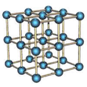
It is hard to imagine substances much more different than a gas and a solid. It is therefore quite surprising that we can employ our study of gases to accurately understand certain properties of solids. Consider a crystal of atoms of the type shown in the figure. The individual atoms are stuck fast in position: they certainly don’t act like a gas. But the vibrations of the atoms — in other words, sound waves — can be treated using the same formalism that we introduced for photons.

3.3.1 The Debye Model

Quantum mechanics turns electromagnetic waves into discrete packets of energy called photons. In exactly the same way, sounds waves in solids also come in discrete packets. They are called phonons. We’ll take the energy of a phonon to again be of the form

\displaystyle E=\hbar\omega=\hbar kc_{s}

(3.101)

where $c_{s}$ is now the speed of sound rather than the speed of light.

The density of states for phonons is the same as that of photons (3.95) with two exceptions: we must replace the speed of light $c$ with the speed of sound $c_{s}$ ; and phonons have three polarization states rather than two. There are two transverse polarizations (like the photon) but also a longitudinal mode. The density of states is therefore

\displaystyle g(\omega)d\omega=\frac{3V}{2\pi^{2}c_{s}^{3}}\omega^{2}d\omega

There is one further important difference between phonons and photons. While light waves can have arbitrarily high frequency, sound waves cannot. This is because high frequency waves have small wavelengths, $\lambda=2\pi c_{s}/\omega$ . But there is a minimum wavelength in the problem set by the spacing between atoms. it is not possible for sound waves to propagate through a solid with wavelength smaller than the atomic spacing because there’s nothing in the middle there to shake.

We will denote the maximum allowed phonon frequency as $\omega_{D}$ . The minimum wavelength, $\lambda_{D}$ , should be somewhere around the lattice spacing between atoms, which is $(V/N)^{1/3}$ , so we expect that $\omega_{D}\sim(N/V)^{1/3}c_{s}$ . But how can we work out the coefficient? There is a rather clever argument to determine $\omega_{D}$ due to Debye. (So clever that he gets his initial on the frequency and his name on the section heading). We start by counting the number of single phonon states,

\displaystyle\int^{\omega_{D}}_{0}d\omega\ g(w)=\frac{V\omega_{D}^{3}}{2\pi^{2% }c_{s}^{3}}

The clever bit of the argument is to identify this with the number of degrees of freedom in the solid. This isn’t immediately obvious. The number of degrees of freedom in a lattice of $N$ atoms is $3N$ since each atom can move in three directions. But the number of single phonon states is counting collective vibrations of all the atoms together. Why should they be equal?

To really see what’s going on, one should compute the correct energy eigenstates of the lattice and just count the number of single phonon modes with wavevectors inside the first Brillouin zone. (You can learn about Brillouin zones in the Applications of Quantum Mechanics lecture notes.) But to get the correct intuition, we can think in the following way: in general the solid will have many phonons inside it and each of these phonons could sit in any one of the single-phonon states that we counted above. Suppose that there are three phonons sitting in the same state. We say that this state is occupied three times. In this language, each of the states above can be occupied an arbitrary number of times, restricted only by the energy available. If you want to describe the total state of the system, you need to say how many phonons are in the first state, and how many are in the second state and so on. The number of one-phonon states is then playing the role of the number of degrees of freedom: it is the number of things you can excite.

The net result of this argument is to equate

\displaystyle 3N=\frac{V\omega_{D}^{3}}{2\pi^{2}c_{s}^{3}}\ \ \ \Rightarrow\ % \ \ \omega_{D}=\left(\frac{6\pi^{2}N}{V}\right)^{1/3}c_{s}

We see that $\omega_{D}$ is related to the atomic spacing $(V/N)^{1/3}$ as we anticipated above, but now we have the coefficient too. However, in some sense, the argument of Debye is “answer analysis”. It was constructed to ensure that we have the right high-temperature behaviour that we will see below.

From the maximum frequency $\omega_{D}$ we can construct an associated energy scale, $\hbar\omega_{D}$ , and temperature scale,

\displaystyle T_{D}=\frac{\hbar\omega_{D}}{k_{B}}

This is known as the Debye temperature. It provides a way of characterising all solids: it is the temperature at which the highest frequency phonon starts to become excited. $T_{D}$ ranges from around $100K$ for very soft materials such as lead through to $2000K$ for hard materials such as diamond. Most materials have Debye temperatures around room temperature ( $\pm 100K$ or so).

Heat Capacity of Solids

All that remains is to put the pieces together. Like photons, the number of phonons is not conserved. The partition function for phonons of a fixed frequency, $\omega$ , is the same as for photons (3.96),

\displaystyle Z_{\omega}=1+e^{-\beta\hbar\omega}+e^{-2\beta\hbar\omega}+\ldots% =\frac{1}{1-e^{-\beta\hbar\omega}}

Summing over all frequencies, the partition function is then

\displaystyle\log Z_{\rm phonon}=\int_{0}^{\omega_{D}}d\omega\ g(\omega)\log Z% _{\omega}

where the partition function $Z_{\omega}$ for a single phonon of frequency $\omega$ is the same as that of a photon (3.96). The total energy in sound waves is therefore

\displaystyle E=\int_{0}^{\omega_{D}}d\omega\ \frac{\hbar\omega g(\omega)}{e^{% \beta\hbar\omega}-1}=\frac{3V\hbar}{2\pi^{2}c_{s}^{3}}\int_{0}^{\omega_{D}}d% \omega\frac{\omega^{3}}{e^{\beta\hbar\omega}-1}

Figure 16: Experimental data for heat capacities. The solid line is the Debye prediction. (Source: D. Schroeder An Introduction to Thermal Physics)

We again rescale the integration variable to $x=\beta\hbar\omega$ so the upper limit of the integral becomes $x_{D}=T_{D}/T$ . Then we have

\displaystyle E=\frac{3V}{2\pi^{2}(\hbar c_{s})^{3}}(k_{B}T)^{4}\int_{0}^{T_{D% }/T}dx\ \frac{x^{3}}{e^{x}-1}

The integral is a function of $T_{D}/T$ . It has no analytic expression. However, we can look in the two extremes. Firstly, for $T\ll T_{D}$ we can replace the upper limit of the integral by infinity. We’re then left with the same definite integral that we appeared for photons, $I=\int^{\infty}dx\ x^{3}/(e^{x}-1)=\pi^{4}/15$ . In this low-temperature regime, the heat capacity is proportional to $T^{3}$ ,

\displaystyle C_{V}=\frac{\partial{E}}{\partial{T}}=\frac{2\pi^{2}Vk_{B}^{4}}{% 5\hbar^{3}c_{s}^{3}}\,T^{3}\ \ \ \ \ \ \ \ \ (T\ll T_{D})

(3.102)

It is often expressed in terms of the Debye temperature $T_{D}$ , so it reads

\displaystyle C_{V}=Nk_{B}\frac{12\pi^{4}}{5}\left(\frac{T}{T_{D}}\right)^{3}

(3.103)

In contrast, at temperatures $T\gg T_{D}$ we only integrate over small values of $x$ , allowing us to Taylor expand the integrand,

\displaystyle\int_{0}^{T_{D}/T}dx\ \frac{x^{3}}{e^{x}-1}=\int^{T_{D}/T}_{0}dx% \ \left(x^{2}+\ldots\right)=\frac{1}{3}\left(\frac{T_{D}}{T}\right)^{3}+\ldots

This ensures that the energy grows linearly with $T$ and the heat capacity tends towards a constant value

\displaystyle C_{V}=\frac{Vk_{B}^{4}T_{D}^{3}}{2\pi^{2}\hbar^{3}c_{s}^{3}}=3Nk% _{B}\ \ \ \ \ \ \ \ \ (T\gg T_{D})

(3.104)

This high-temperature behaviour has been known experimentally since the early 1800’s. It is called the Dulong-Petit law. Debye’s argument for the value of $\omega_{D}$ was basically constructed to reproduce the coefficient $3N$ in the formula above. This was known experimentally, but also from an earlier model of vibrations in a solid due to Einstein. (You met the Einstein model in the first problem sheet). Historically, the real success of the Debye model was the correct prediction of the $T^{3}$ behaviour of $C_{V}$ at low temperatures.

In most materials the heat capacity is dominated by the phonon contribution. (In metals there is an additional contribution from conduction electrons that we will calculate in Section 3.6). The heat capacity of three materials is shown in Figure 16, together with the predictions from the Debye model. As you can see, it works very well! The deviation from theory at high temperatures is due to differences between $C_{V}$ and $C_{p}$ , the heat capacity at constant pressure.

What’s Wrong with the Debye Model?

As we’ve seen, the Debye model is remarkably accurate in capturing the heat capacities of solids. Nonetheless, it is a caricature of the physics. The most glaring problem is our starting point (3.101). The relationship $E=\hbar\omega$ between energy and frequency is fine; the mistake is the relationship between frequency $\omega$ and wavevector (or momentum) $k$ , namely $\omega=kc_{s}$ . Equations of this type, relating energy and momentum, are called dispersion relations. It turns out that that the dispersion relation for phonons is a little more complicated.

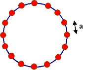
It is not hard to compute the dispersion relation for phonons. (You will, in fact, do this calculation in the Applications of Quantum Mechanics course). For simplicity, we’ll work with a one dimensional periodic lattice of $N$ atoms as shown in the figure. The equilibrium position of each atom is $x_{l}=la$ and we impose periodic boundary conditions by insisting that $x_{N+1}\equiv x_{1}$ . Let $u_{l}$ be the deviation from equilibrium, $u_{l}=x_{l}-la$ . If we approximate the bonds joining the atoms as harmonic oscillators, the Hamiltonian governing the vibrations is

\displaystyle H=\frac{1}{2m}\sum_{i}\dot{u}_{i}^{2}+\frac{\alpha}{2}\sum_{i}(u% _{i}-u_{i+1})^{2}

where $\alpha$ is a parameter governing the strength of the bonds between atoms. The equation of motion is

\displaystyle\ddot{u_{i}}=\frac{\alpha}{m}(2u_{i}-u_{i+1}-u_{i-1})

This is easily solved by the discrete Fourier transform. We make the ansatz

\displaystyle u_{l}=\frac{1}{\sqrt{N}}\sum_{k}\tilde{u}_{k}e^{i(kla-\omega_{k}% t)}

Plugging this into the equation of motion gives the dispersion relation

\displaystyle\omega_{k}=2\sqrt{\frac{\alpha}{m}}\left|\sin\left(\frac{ka}{2}% \right)\right|

To compute the partition function correctly in this model, we would have to revisit the density of states using the new dispersion relation $E(k)=\hbar\omega_{k}$ . The resulting integrals are messy. However, at low temperatures only the smallest frequency modes are excited and, for small $k a$ , the $\sin$ function is approximately linear. This means that we get back to the dispersion relation that we used in the Debye model, $\omega=kc_{s}$ , with the speed of sound given by $c_{s}=a\sqrt{\alpha/m}$ . Moreover, at very high temperatures it is simple to check that this model gives the Dulong-Petit law as expected. It deviates from the Debye model only at intermediate temperatures and, even here, this deviation is mostly negligible.

3.4 The Diatomic Gas Revisited

With a bit of quantum experience under our belt, we can look again at the diatomic gas that we discussed in Section 2.4. Recall that the classical prediction for the heat capacity — $C_{V}=\frac{7}{2}Nk_{B}$ — only agrees with experiment at very high temperatures. Instead, the data suggests that as the temperature is lowered, the vibrational modes and the rotational modes become frozen out. But this is exactly the kind of behaviour that we expect for a quantum system where there is a minimum energy necessary to excite each degree of freedom. Indeed, this “freezing out” of modes saved us from ultra-violet catastrophe in the case of blackbody radiation and gave rise to a reduced heat capacity at low temperatures for phonons.

Let’s start with the rotational modes, described by the Hamiltonian (2.66). Treating this as a quantum Hamiltonian, it has energy levels

\displaystyle E=\frac{\hbar^{2}}{2I}j(j+1)\ \ \ \ j=0,1,2,\ldots

The degeneracy of each energy level is $2j+1$ . Thus the rotational partition function for a single molecule is

\displaystyle Z_{\rm rot}=\sum_{j=0}^{\infty}(2j+1)e^{-\beta\hbar^{2}j(j+1)/2I}

When $T\gg\hbar^{2}/2Ik_{B}$ , we can approximate the sum by the integral to get

\displaystyle Z_{\rm rot}\approx\int_{0}^{\infty}dx\ (2x+1)e^{-\beta\hbar^{2}x% (x+1)/2I}=\frac{2I}{\beta\hbar^{2}}

which agrees with our result for the classical partition function (2.67).

In contrast, for $T\ll\hbar^{2}/2Ik_{B}$ all states apart from $j=0$ effectively decouple and we have simply $Z_{\rm rot}\approx 1$ . At these temperatures, the rotational modes are frozen at temperatures accessible in experiment so only the translational modes contribute to the heat capacity.

This analysis also explains why there is no rotational contribution to the heat capacity of a monatomic gas. One could try to argue this away by saying that atoms are point particles and so can’t rotate. But this simply isn’t true. The correct argument is that the moment of inertia $I$ of an atom is very small and the rotational modes are frozen. Similar remarks apply to rotation about the symmetry axis of a diatomic molecule.

The vibrational modes are described by the harmonic oscillator. You already computed the partition function for this on the first examples sheet (and, in fact, implicitly in the photon and phonon calculations above). The energies are

\displaystyle E=\hbar\omega(n+\frac{1}{2})

and the partition function is

\displaystyle Z_{\rm vib}=\sum_{n}e^{-\beta\hbar\omega(n+\frac{1}{2})}=e^{-% \beta\hbar\omega/2}\sum_{n}e^{-\beta\hbar\omega n}=\frac{e^{-\beta\hbar\omega/% 2}}{1-e^{-\beta\hbar\omega}}=\frac{1}{2\sinh(\beta\hbar\omega/2)}

At high temperatures $\beta\hbar\omega\ll 1$ , we can approximate the partition function as $Z_{\rm vib}\approx 1/\beta\hbar\omega$ which again agrees with the classical result (2.68). At low temperatures $\beta\hbar\omega\gg 1$ , the partition function becomes $Z_{\rm vib}\approx e^{-\beta\hbar\omega/2}$ . This is a contribution from the zero-point energy of the harmonic oscillator. It merely gives the expected additive constant to the energy per particle,

\displaystyle E_{\rm vib}=-\frac{\partial}{\partial{\beta}}\log Z_{\rm vib}% \approx\frac{\hbar\omega}{2}

and doesn’t contribute the heat capacity. Once again, we see how quantum effects explain the observed behaviour of the heat capacity of the diatomic gas. The end result is a graph that looks like that shown in Figure 11.

3.5 Bosons

For the final two topics of this section, we will return again to the simple monatomic ideal gas. The classical treatment that we described in Section 2.2 has limitations. As the temperature decreases, the thermal de Broglie wavelength,

\displaystyle\lambda=\sqrt{\frac{2\pi\hbar^{2}}{mk_{B}T}}

gets larger. Eventually it becomes comparable to the inter-particle separation, $(V/N)^{1/3}$ . At this point, quantum effects become important. If the particles are non-interacting, there is really only one important effect that we need to consider: quantum statistics.

Recall that in quantum mechanics, particles come in two classes: bosons and fermions. Which class a given particle falls into is determined by its spin, courtesy of the spin-statistics theorem. Integer spin particles are bosons. This means that any wavefunction must be symmetric under the exchange of two particles,

\displaystyle\psi(\vec{r}_{1},\vec{r}_{2})=\psi(\vec{r}_{2},\vec{r}_{1})

Particles with ${\textstyle\frac{1}{2}}$ -integer spin are fermions. They have an anti-symmetrized wavefunction,

\displaystyle\psi(\vec{r}_{1},\vec{r}_{2})=-\psi(\vec{r}_{2},\vec{r}_{1})

At low temperatures, the behaviour of bosons and fermions is very different. All familiar fundamental particles such as the electron, proton and neutron are fermions. But an atom that contains an even number of fermions acts as a boson as long as we do not reach energies large enough to dislodge the constituent particles from their bound state. Similarly, an atom consisting of an odd number of electrons, protons and neutrons will be a fermion. (In fact, the proton and neutron themselves are not fundamental: they are fermions because they contain three constituent quarks, each of which is a fermion. If the laws of physics were different so that four quarks formed a bound state rather than three, then both the proton and neutron would be bosons and, as we will see in the next two sections, nuclei would not exist!).

We will begin by describing the properties of bosons and then turn to a discussion of fermions to Section 3.6.

3.5.1 Bose-Einstein Distribution

We’ll change notation slightly from earlier sections and label the single particle quantum states of the system by $|r\rangle$ . (We used $|n\rangle$ previously, but $n$ will be otherwise occupied for most of this section). The single particle energies are then $E_{r}$ and we’ll assume that our particles are non-interacting. In that case, you might think that to specify the state of the whole system, you would need to say which state particle 1 is in, and which state particle 2 is in, and so on. But this is actually too much information because particle 1 and particle 2 are indistinguishable. To specify the state of the whole system, we don’t need to attach labels to each particle. Instead, it will suffice to say how many particles are in state 1 and how many particles are in state 2 and so on.

We’ll denote the number of particles in state $|r\rangle$ as $n_{r}$ . If we choose to work in the canonical ensemble, we must compute the partition function,

\displaystyle Z=\sum_{\{n_{r}\}}e^{-\beta n_{r}E_{r}}

where the sum is over all possible ways of partitioning $N$ particles into sets $\{n_{r}\}$ subject to the constraint that $\sum_{r}n_{r}=N$ . Unfortunately, the need to impose this constraint makes the sums tricky. This means that the canonical ensemble is rather awkward when discussing indistinguishable particles. It turns out to be much easier to work in the grand canonical ensemble where we introduce a chemical potential $\mu$ and allow the total number of particles $N$ to fluctuate.

Life is simplest it we think of each state $|r\rangle$ in turn. In the grand canonical ensemble, a given state can be populated by an arbitrary number of particles. The grand partition function for this state is

\displaystyle{\cal Z}_{r}=\sum_{n_{r}}e^{-\beta n_{r}(E_{r}-\mu)}=\frac{1}{1-e% ^{-\beta(E_{r}-\mu)}}

Notice that we’ve implicitly assumed that the sum above converges, which is true only if $(E_{r}-\mu)>0$ . But this should be true for all states $E_{r}$ . We will set the ground state to have energy $E_{0}=0$ , so the grand partition function for a Bose gas only makes sense if

\displaystyle\mu<0

(3.105)

Now we use the fact that all the occupation of one state is independent of any other. The full grand partition function is then

\displaystyle{\cal Z}=\prod_{r}\frac{1}{1-e^{-\beta(E_{r}-\mu)}}

From this we can compute the average number of particles,

\displaystyle N=\frac{1}{\beta}\frac{\partial}{\partial{\mu}}\log{\cal Z}=\sum% _{r}\frac{1}{e^{\beta(E_{r}-\mu)}-1}\equiv\sum_{r}\langle n_{r}\rangle

Here $\langle n_{r}\rangle$ denotes the average number of particles in the state $|r\rangle$ ,

\displaystyle\langle n_{r}\rangle=\frac{1}{e^{\beta(E_{r}-\mu)}-1}

(3.106)

This is the Bose-Einstein distribution. In what follows we will always be interested in the thermodynamic limit where fluctuations around the average are negligible. For this reason, we will allow ourselves to be a little sloppy in notation and we write the average number of particles in $|r\rangle$ as $n_{r}$ instead of $\langle n_{r}\rangle$ .

Notice that we’ve seen expressions of the form (3.106) already in the calculations for photons and phonons — see, for example, equation (3.96). This isn’t coincidence: both photons and phonons are bosons and the origin of this term in both calculations is the same: it arises because we sum over the number of particles in a given state rather than summing over the states for a single particle. As we mentioned in the Section on blackbody radiation, it is not really correct to think of photons or phonons in the grand canonical ensemble because their particle number is not conserved. Nonetheless, the equations are formally equivalent if one just sets $\mu=0$ .

In what follows, it will save ink if we introduce the fugacity

\displaystyle z=e^{\beta\mu}

(3.107)

Since $\mu<0$ , we have $0<z<1$ .

Ideal Bose Gas

Let’s look again at a gas of non-relativistic particles, now through the eyes of quantum mechanics. The energy is

\displaystyle E=\frac{\hbar^{2}k^{2}}{2m}

As explained in Section 3.1, we can replace the sum over discrete momenta with an integral over energies as long as we correctly account for the density of states. This was computed in (3.91) and we reproduce the result below:

\displaystyle g(E)=\frac{V}{4\pi^{2}}\left(\frac{2m}{\hbar^{2}}\right)^{3/2}E^% {1/2}

(3.108)

From this, together with the Bose-Einstein distribution, we can easily compute the total number of particles in the gas,

\displaystyle N=\int dE\ \frac{g(E)}{z^{-1}e^{\beta E}-1}\ ,

(3.109)

There is an obvious, but important, point to be made about this equation. If we can do the integral (and we will shortly) we will have an expression for the number of particles in terms of the chemical potential and temperature: $N=N(\mu,T)$ . That means that if we keep the chemical potential fixed and vary the temperature, then $N$ will change. But in most experimental situations, $N$ is fixed and we’re working in the grand canonical ensemble only because it is mathematically simpler. But nothing is for free. The price we pay is that we will have to invert equation (3.109) to get it in the form $\mu=\mu(N,T)$ . Then when we change $T$ , keeping $N$ fixed, $\mu$ will change too. We have already seen an example of this in the ideal gas where the chemical potential is given by (2.62).

The average energy of the Bose gas is,

\displaystyle E=\int dE\ \frac{Eg(E)}{z^{-1}e^{\beta E}-1}\ ,

(3.110)

And, finally, we can compute the pressure. In the grand canonical ensemble this is,

\displaystyle pV=\frac{1}{\beta}\log{\cal Z}=-\frac{1}{\beta}\int dE\,g(E)\log% \left(1-ze^{-\beta E}\right)

We can manipulate this last expression using an integration by parts. Because $g(E)\sim E^{1/2}$ , this becomes

\displaystyle pV=\frac{2}{3}\int dE\ \frac{Eg(E)}{z^{-1}e^{\beta E}-1}=\frac{2% }{3}E

(3.111)

This is implicitly the equation of state. But we still have a bit of work to do. Equation (3.110) gives us the energy as a function of $\mu$ and $T$ . And, by the time we have inverted (3.109), it gives us $\mu$ as a function of $N$ and $T$ . Substituting both of these into (3.111) will give the equation of state. We just need to do the integrals…

3.5.2 A High Temperature Quantum Gas is (Almost) Classical

Unfortunately, the integrals (3.109) and (3.110) look pretty fierce. Shortly, we will start to understand some of their properties, but first we look at a particularly simple limit. We will expand the integrals (3.109), (3.110) and (3.111) in the limit $z=e^{\beta\mu}\ll 1$ . We’ll figure out the meaning of this expansion shortly (although there’s a clue in the title of this section if you’re impatient). Let’s look at the particle density (3.109),

$\displaystyle\frac{N}{V}$	$\displaystyle=$	$\displaystyle\frac{1}{4\pi^{2}}\left(\frac{2m}{\hbar^{2}}\right)^{3/2}\int_{0}% ^{\infty}dE\ \frac{E^{1/2}}{z^{-1}e^{\beta E}-1}$
	$\displaystyle=$	$\displaystyle\frac{1}{4\pi^{2}}\left(\frac{2m}{\hbar^{2}}\right)^{3/2}\int_{0}% ^{\infty}dE\ \frac{ze^{-\beta E}E^{1/2}}{1-ze^{-\beta E}}$
	$\displaystyle=$	$\displaystyle\frac{1}{4\pi^{2}}\left(\frac{2m}{\hbar^{2}}\right)^{3/2}\,\frac{% z}{\beta^{3/2}}\int_{0}^{\infty}dx\ \sqrt{x}e^{-x}(1+ze^{-x}+\ldots)$

where we made the simple substitution $x=\beta E$ . The integrals are all of the Gaussian type and can be easily evaluated by making one further substitution $x=u^{2}$ . The final answer can be conveniently expressed in terms of the thermal wavelength $\lambda$ ,

\displaystyle\frac{N}{V}=\frac{z}{\lambda^{3}}\left(1+\frac{z}{2\sqrt{2}}+% \ldots\right)

(3.112)

Now we’ve got the answer, we can ask what we’ve done! What kind of expansion is $z\ll 1$ ? From the above expression, we see that the expansion is consistent only if $\lambda^{3}N/V\ll 1$ , which means that the thermal wavelength is much less than the interparticle spacing. But this is true at high temperatures: the expansion $z\ll 1$ is a high temperature expansion.

At first glance, it is surprising that $z=e^{\beta\mu}\ll 1$ corresponds to high temperatures. When $T\rightarrow\infty$ , $\beta\rightarrow 0$ so naively it looks as if $z\rightarrow 1$ . But this is too naive. If we keep the particle number $N$ fixed in (3.109) then $\mu$ must vary as we change the temperature, and it turns out that $\mu\rightarrow-\infty$ faster than $\beta\rightarrow 0$ . To see this, notice that to leading order we need $z/\lambda^{3}$ to be constant, so $z\sim T^{-3/2}$ .

High Temperature Equation of State of a Bose Gas

We now wish to compute the equation of state. We know from (3.111) that $pV={\textstyle\frac{2}{3}}E$ . So we need to compute $E$ using the same $z\ll 1$ expansion as above. From (3.110), the energy density is

$\displaystyle\frac{E}{V}$	$\displaystyle=$	$\displaystyle\frac{1}{4\pi^{2}}\left(\frac{2m}{\hbar^{2}}\right)^{3/2}\int_{0}% ^{\infty}dE\ \frac{E^{3/2}}{z^{-1}e^{\beta E}-1}$	(3.113)
	$\displaystyle=$	$\displaystyle\frac{1}{4\pi^{2}}\left(\frac{2m}{\hbar^{2}}\right)^{3/2}\,\frac{% z}{\beta^{5/2}}\int_{0}^{\infty}dx\ {x}^{3/2}e^{-x}(1+ze^{-x}+\ldots)$
	$\displaystyle=$	$\displaystyle\frac{3z}{2\lambda^{3}\beta}\left(1+\frac{z}{4\sqrt{2}}+\ldots\right)$

The next part’s a little fiddly. We want to eliminate $z$ from the expression above in favour of $N/V$ . To do this we invert (3.112), remembering that we’re working in the limit $z\ll 1$ and $\lambda^{3}N/V\ll 1$ . This gives

\displaystyle z=\frac{\lambda^{3}N}{V}\left(1-\frac{1}{2\sqrt{2}}\frac{\lambda% ^{3}N}{V}+\ldots\right)

which we then substitute into (3.113) to get

\displaystyle E=\frac{3}{2}\frac{N}{\beta}\left(1-\frac{1}{2\sqrt{2}}\frac{% \lambda^{3}N}{V}+\ldots\right)\left(1+\frac{1}{4\sqrt{2}}\frac{\lambda^{3}N}{V% }+\ldots\right)

and finally we substitute this into $pV={\textstyle\frac{2}{3}}E$ to get the equation of state of an ideal Bose gas at high temperatures,

\displaystyle pV=Nk_{B}T\left(1-\frac{\lambda^{3}N}{4\sqrt{2}V}+\ldots\right)

(3.114)

which reproduces the classical ideal gas, together with a term that we can identify as the second virial coefficient in the expansion (2.69). However, this correction to the pressure hasn’t arisen from any interactions among the atoms: it is solely due to quantum statistics. We see that the effect of bosonic statistics on the high temperature gas is to reduce the pressure.

3.5.3 Bose-Einstein Condensation

We now turn to the more interesting question: what happens to a Bose gas at low temperatures? Recall that for convergence of the grand partition function we require $\mu<0$ so that $z=e^{\beta\mu}\in(0,1)$ . Since the high temperature limit is $z\rightarrow 0$ , we’ll anticipate that quantum effects and low temperatures come about as $z\rightarrow 1$ .

Recall that the number density is given by (3.109) which we write as

\displaystyle\frac{N}{V}=\frac{1}{4\pi^{2}}\left(\frac{2mk_{B}T}{\hbar^{2}}% \right)^{3/2}\int_{0}^{\infty}dx\ \frac{x^{1/2}}{z^{-1}e^{x}-1}\equiv\frac{1}{% \lambda^{3}}\,g_{3/2}(z)

(3.115)

where the function $g_{3/2}(z)$ is one of a class of functions which appear in the story of Bose gases,

\displaystyle g_{n}(z)=\frac{1}{\Gamma(n)}\int_{0}^{\infty}dx\ \frac{x^{n-1}}{% z^{-1}e^{x}-1}

(3.116)

These functions are also known as polylogarithms and sometimes denoted as $Li_{n}(z)=g_{n}(z)$ . The function $g_{3/2}$ is relevant for the particle number and the function $g_{5/2}$ appears in the calculation of the energy in (3.110). For reference, the gamma function has value $\Gamma(3/2)=\sqrt{\pi}/2$ . (Do not confuse these functions $g_{n}(z)$ with the density of states $g(E)$ . They are not related; they just share a similar name).

In Section 3.5.2 we looked at (3.115) in the $T\rightarrow\infty$ limit. There we saw that $\lambda\rightarrow 0$ but the function $g_{3/2}(z)\rightarrow 0$ in just the right way to compensate and keep $N/V$ fixed. What now happens in the other limit, $T\rightarrow 0$ and $\lambda\rightarrow\infty$ . One might harbour the hope that $g_{3/2}(z)\rightarrow\infty$ and again everything balances nicely with $N/V$ remaining constant. We will now show that this can’t happen.

A couple of manipulations reveals that the integral (3.116) can be expressed in terms of a sum,

$\displaystyle g_{n}(z)$	$\displaystyle=$	$\displaystyle\frac{1}{\Gamma(n)}\int dx\ \frac{zx^{n-1}e^{-x}}{1-ze^{-x}}$
	$\displaystyle=$	$\displaystyle\frac{1}{\Gamma(n)}z\int dx\ x^{n-1}e^{-x}\sum_{m=0}^{\infty}z^{m% }e^{-mx}$
	$\displaystyle=$	$\displaystyle\frac{1}{\Gamma(n)}\sum_{m=1}^{\infty}z^{m}\int dx\ x^{n-1}e^{-mx}$
	$\displaystyle=$	$\displaystyle\frac{1}{\Gamma(n)}\sum_{m=1}^{\infty}\frac{z^{m}}{m^{n}}\int du% \ u^{n-1}e^{-u}$

But the integral that appears in the last line above is nothing but the definition of the gamma function $\Gamma(n)$ . This means that we can write

\displaystyle g_{n}(z)=\sum_{m=1}^{\infty}\frac{z^{m}}{m^{n}}

(3.117)

We see that $g_{n}(z)$ is a monotonically increasing function of $z$ . Moreover, at $z=1$ , it is equal to the Riemann zeta function

\displaystyle g_{n}(1)=\zeta(n)

For our particular problem it will be useful to know that $\zeta(3/2)\approx 2.612$ .

Let’s now return to our story. As we decrease $T$ in (3.115), keeping $N/V$ fixed, $z$ and hence $g_{3/2}(z)$ must both increase. But $z$ can’t take values greater than 1. When we reach $z=1$ , let’s denote the temperature as $T=T_{c}$ . We can determine $T_{c}$ by setting $z=1$ in equation (3.115),

\displaystyle T_{c}=\left(\frac{2\pi\hbar^{2}}{k_{B}m}\right)\left(\frac{1}{% \zeta(3/2)}\frac{N}{V}\right)^{2/3}

(3.118)

What happens if we try to decrease the temperature below $T_{c}$ ? Taken at face value, equation (3.115) tells us that the number of particles should decrease. But that’s a stupid conclusion! It says that we can make particles disappear by making them cold. Where did they go? We may be working in the grand canonical ensemble, but in the thermodynamic limit we expect $\Delta N\sim 1/\sqrt{N}$ which is too small to explain our missing particles. Where did we misplace them? It looks as if we made a mistake in the calculation.

In fact, we did make a mistake in the calculation. It happened right at the beginning. Recall that back in Section 3.1 we replaced the sum over states with an integral over energies,

\displaystyle\sum_{\vec{k}}\approx\frac{V(2m)^{3/2}}{4\pi^{2}\hbar^{3}}\int dE% \ E^{1/2}

Because of the weight $\sqrt{E}$ in the integrand, the ground state with $E=0$ doesn’t contribute to the integral. We can use the Bose-Einstein distribution (3.106) to compute the number of states that we expect to be missing because they sit in this $E=0$ ground state,

\displaystyle n_{0}=\frac{1}{z^{-1}-1}

(3.119)

For most values of $z\in(0,1)$ , there are just a handful of particles sitting in this lowest state and it doesn’t matter if we miss them. But as $z$ gets very very close to 1 (meaning $z\approx 1-1/N$ ) then we get a macroscopic number of particles occupying the ground state.

It is a simple matter to redo our calculation taking into account the particles in the ground state. Equation (3.115) is replaced by

\displaystyle N=\frac{V}{\lambda^{3}}\,g_{3/2}(z)+\frac{z}{1-z}

Now there’s no problem keeping $N$ fixed as we take $z$ close to 1 because the additional term diverges. This means that if we have finite $N$ , then as we decrease $T$ we can never get to $z=1$ . Instead, $z$ must level out around $z\approx 1-1/N$ as $T\rightarrow 0$ .

For $T<T_{c}$ , the number of particles sitting in the ground state is $\cal{O}(N)$ . Some simple algebra allows us to determine that fraction of particles in the ground state is

\displaystyle\frac{n_{0}}{N}=1-\frac{V}{N\lambda^{3}}\,\zeta(3/2)=1-\left(% \frac{T}{T_{c}}\right)^{3/2}

(3.120)

At temperatures $T<T_{c}$ , a macroscopic number of atoms discard their individual identities and merge into a communist collective, a single quantum state so large that it can be seen with the naked eye. This is known as the Bose-Einstein condensate. It provides an exquisitely precise playground in which many quantum phenomena can be tested.

Bose-Einstein Condensates in the Lab

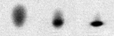
Bose-Einstein condensates (often shortened to BECs) of weakly interacting atoms were finally created in 1995, some 70 years after they were first predicted. These first BECs were formed of Rubidium, Sodium or Lithium and contained between $N\sim 10^{4}\rightarrow 10^{7}$ atoms. The transition temperatures needed to create these condensates are extraordinarily small, around $T_{c}\sim 10^{-7}K$ . Figure 19 shows the iconic colour enhanced plots that reveal the existence of the condensate. To create these plots, the atoms are stored in a magnetic trap which is then turned off. A picture is taken of the atom cloud a short time $t$ later when the atoms have travelled a distance $\hbar kt/m$ . The grey UFO-like smudges above are the original pictures. From the spread of atoms, the momentum distribution of the cloud is inferred and this is what is shown in Figure 19. The peak that appears in the last two plots reveals that a substantial number of atoms were indeed sitting in the momentum ground state. (This is not a $k=0$ state because of the finite trap and the Heisenberg uncertainty relation). The initial discoverers of BECs, Eric Cornell and Carl Wieman from Boulder and Wolfgang Ketterle from MIT, were awarded the 2001 Nobel prize in physics.

Figure 19: The velocity distribution of Rubidium atoms, taken from the Ketterle lab at MIT. The left-hand picture shows

T>T_{c}

, just before the condensate forms. The middle and right-hand pictures both reveal the existence of the condensate.

Low Temperature Equation of State of a Bose Gas

The pressure of the ideal Bose gas was computed in (3.111). We can express this in terms of our new favourite functions (3.116) as

\displaystyle p=\frac{2}{3}\frac{E}{V}=\frac{k_{B}T}{\lambda^{3}}\,g_{5/2}(z)

(3.121)

Formally there is also a contribution from the ground state, but it is $\log(1-z)/V$ which is a factor of $N$ smaller than the term above and can be safely ignored. At low temperatures, $T<T_{c}$ , we have $z\approx 1$ and

\displaystyle p=\frac{k_{B}T}{\lambda^{3}}\zeta(5/2)

So at low temperatures, the equation of state of the ideal Bose gas is very different from the classical, high temperature, behaviour. The pressure scales as $p\sim T^{5/2}$ (recall that there is a factor of $T^{3/2}$ lurking in the $\lambda$ ). More surprisingly, the pressure is independent of the density of particles $N/V$ .

3.5.4 Heat Capacity: Our First Look at a Phase Transition

Let’s try to understand in more detail what happens as we pass through the critical temperature $T_{c}$ . We will focus on how the heat capacity behaves on either side of the critical temperature.

We’ve already seen in (3.121) that we can express the energy in terms of the function $g_{5/2}(z)$ ,

\displaystyle\frac{E}{V}=\frac{3}{2}\frac{k_{B}T}{\lambda^{3}}\,g_{5/2}(z)

so the heat capacity becomes

\displaystyle\frac{C_{V}}{V}=\frac{1}{V}\frac{dE}{dT}=\frac{15k_{B}}{4\lambda^% {3}}g_{5/2}(z)+\frac{3}{2}\frac{k_{B}T}{\lambda^{3}}\frac{dg_{5/2}}{dz}\frac{% dz}{dT}

(3.122)

The first term gives a contribution both for $T<T_{c}$ and for $T>T_{c}$ . However, the second term includes a factor of $dz/dT$ and $z$ is a very peculiar function of temperature: for $T>T_{c}$ , it is fairly smooth, dropping off at $T=T_{c}$ . However, as $T\rightarrow T_{c}$ , the fugacity rapidly levels off to the value $z\approx 1-1/N$ . For $T<T_{c}$ , $z$ doesn’t change very much at all. The net result of this is that the second term only contributes when $T>T_{c}$ . Our goal here is to understand how this contribution behaves as we approach the critical temperature.

Let’s begin with the easy bit. Below the critical temperature, $T<T_{c}$ , only the first term in (3.122) contributes and we may happily set $z=1$ . This gives the heat capacity,

\displaystyle C_{V}=\frac{15Vk_{B}}{4\lambda^{3}}\zeta(5/2)\sim T^{3/2}

(3.123)

Now we turn to $T>T_{c}$ . Here we have $z<1$ , so $g_{5/2}(z)<g_{5/2}(1)$ . We also have $dz/dT<0$ . This means that the heat capacity decreases for $T>T_{c}$ . But we know that for $T<T_{c}$ , $C_{V}\sim T^{3/2}$ so the heat capacity must have a maximum at $T=T_{c}$ . Our goal in this section is to understand a little better what the function $C_{V}$ looks like in this region.

To compute the second term in (3.122) we need to understand both $g^{\prime}_{5/2}$ and how $z$ changes with $T$ as we approach $T_{c}$ from above. The first calculation is easy is we use our expression (3.117),

\displaystyle g_{n}(z)=\sum_{m=1}^{\infty}\frac{z^{m}}{m^{n}}\ \ \ \Rightarrow% \ \ \ \frac{d}{dz}g_{n}(z)=\frac{1}{z}g_{n-1}(z)

(3.124)

As $T\rightarrow T_{c}$ from above, $dg_{5/2}/dT\rightarrow\zeta(3/2)$ , a constant. All the subtleties lie in the remaining term, $dz/dT$ . After all, this is the quantity which is effectively vanishing for $T<T_{c}$ . What’s it doing at $T>T_{c}$ ? To figure this out is a little more involved. We start with our expression (3.115),

\displaystyle g_{3/2}(z)=\frac{N\lambda^{3}}{V}\ \ \ \ \ T>T_{c}

(3.125)

and we’ll ask what happens to the function $g_{3/2}(z)$ as $z\rightarrow 1$ , keeping $N$ fixed. We know that exactly at $z=1$ , $g_{3/2}(1)=\zeta(3/2)$ . But how does it approach this value? To answer this, it is actually simplest to look at the derivative $dg_{3/2}/dz=g_{1/2}/z$ , where

\displaystyle g_{1/2}(z)=\frac{1}{\Gamma(1/2)}\int_{0}^{\infty}dx\ \frac{x^{-1% /2}}{z^{-1}e^{x}-1}

The reason for doing this is that $g_{1/2}$ diverges as $z\rightarrow 1$ and it is generally easier to isolate divergent parts of a function than some finite piece. Indeed, we can do this straightforwardly for $g_{1/2}$ by looking at the integral very close to $x=0$ , we can write

$\displaystyle g_{1/2}(z)$	$\displaystyle=$	$\displaystyle\frac{1}{\Gamma(1/2)}\int_{0}^{\epsilon}dx\ \frac{x^{-1/2}}{z^{-1% }(1+x)-1}+{\rm finite}$
	$\displaystyle=$	$\displaystyle\frac{z}{\Gamma(1/2)}\int_{0}^{\epsilon}dx\ \frac{x^{-1/2}}{(1-z)% +x}+\ldots$
	$\displaystyle=$	$\displaystyle\frac{2z}{\sqrt{1-z}}\frac{1}{\Gamma(1/2)}\int_{0}^{\epsilon}du\ % \frac{1}{1+u^{2}}+\ldots$

where, in the last line, we made the substution $u=\sqrt{x/(1-z)}$ . So we learn that as $z\rightarrow 1$ , $g_{1/2}(z)\rightarrow z(1-z)^{-1/2}$ . But this is enough information to tell us how $g_{3/2}$ approaches its value at $z=1$ : it must be

\displaystyle g_{3/2}(z)\approx\zeta(3/2)+A(1-z)^{1/2}+\ldots

for some constant $A$ . Inserting this into our equation (3.125) and rearranging, we find that as $T\rightarrow T_{c}$ from above,

$\displaystyle z$	$\displaystyle\approx$	$\displaystyle 1-\frac{1}{A^{2}}\left(\zeta(3/2)-\frac{N\lambda^{3}}{V}\right)^% {2}$
	$\displaystyle=$	$\displaystyle 1-\frac{\zeta(3/2)^{2}}{A^{2}}\left(\left(\frac{T}{T_{c}}\right)% ^{3/2}-1\right)^{2}$
	$\displaystyle\approx$	$\displaystyle 1-B\left(\frac{T-T_{c}}{T_{c}}\right)^{2}$

where, in the second line, we used the expression of the critical temperature (3.118). $B$ is some constant that we could figure out with a little more effort, but it won’t be important for our story. From the expression above, we can now determine $dz/dT$ as $T\rightarrow T_{c}$ . We see that it vanishes linearly at $T=T_{c}$ .

Putting all this together, we can determine the expression for the heat capacity (3.122) when $T>T_{c}$ . We’re not interested in the coefficients, so we’ll package a bunch of numbers of order $1$ into a constant $b$ and the end result is

\displaystyle C_{V}=\frac{15Vk_{B}}{4\lambda^{3}}g_{5/2}(z)-b\left(\frac{T-T_{% c}}{T_{c}}\right)

The first term above goes smoothly over to the expression (3.123) for $C_{V}$ when $T<T_{c}$ . But the second term is only present for $T>T_{c}$ . Notice that it goes to zero as $T\rightarrow T_{c}$ , which ensures that the heat capacity is continuous at this point. But the derivative is not continuous. A sketch of the heat capacity is shown in the figure.

Functions in physics are usually nice and smooth. How did we end up with a discontinuity in the derivative? In fact, if we work at finite $N$ , strictly speaking everything is nice and smooth. There is a similar contribution to $dz/dT$ even at $T<T_{c}$ . We can see that by looking again at the expressions (3.119) and (3.120), which tell us

\displaystyle z=\left(1+\frac{1}{n_{0}}\right)^{-1}=\left(1+\frac{1}{N}\frac{1% }{1-(T/T_{c})^{3/2}}\right)^{-1}\ \ \ \ \ (T<T_{c})

The difference is that while $dz/dT$ is of order one above $T_{c}$ , it is of order $1/N$ below $T_{c}$ . In the thermodynamic limit, $N\rightarrow\infty$ , this results in the discontinuity that we saw above. This is a general lesson: phase transitions with their associated discontinuities can only arise in strictly infinite systems. There are no phase transitions in finite systems.

Superfluid Helium-4

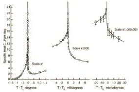
A similar, but much more pronounced, discontinuity is seen in Helium-4 as it becomes a superfluid, a transition which occurs at 2.17 $K$ . The atom contains two protons, two neutrons and two electrons and is therefore a boson. (In contrast, Helium-3 contains just a single neutron and is a fermion). The experimental data for the heat capacity of Helium-4 is shown on the right. The successive graphs are zooming in on the phase transistion: the scales are (from left to right) Kelvin, milliKelvin and microKelvin. The discontinuity is often called the lambda transition on account of the shape of this graph.

There is a close connection between Bose-Einstein condensation described above and superfluids: strictly speaking a non-interacting Bose-Einstein condensate is not a superfluid but superfluidity is a consequence of arbitrarily weak repulsive interactions between the atoms. However, in He-4, the interactions between atoms are strong and the system cannot be described using the simple techniques developed above.

Something very similar to Bose condensation also occurs in superconductivity and superfluidity of Helium-3. Now the primary characters are fermions rather than bosons (electrons in the case of superconductivity). As we will see in the next section, fermions cannot condense. But they may form bound states due to interactions and these effective bosons can then undergo condensation.

3.6 Fermions

For our final topic, we will discuss the fermion gases. Our analysis will focus solely on non-interacting fermions. Yet this simple model provides a (surprisingly) good first approximation to a wide range of systems, including electrons in metals at low temperatures, liquid Helium-3 and white dwarfs and neutron stars.

Fermions are particles with ${\textstyle\frac{1}{2}}$ -integer spin. By the spin-statistics theorem, the wavefunction of the system is required to pick up a minus sign under exchange of any particle,

\displaystyle\psi(\vec{r}_{1},\vec{r}_{2})=-\psi(\vec{r}_{2},\vec{r}_{1})

As a corollory, the wavefunction vanishes if you attempt to put two identical fermions in the same place. This is a reflection of the Pauli exclusion principle which states that fermions cannot sit in the same state. We will see that the low-energy physics of a gas of fermions is entirely dominated by the exclusion principle.

We work again in the grand canonical ensemble. The grand partition function for a single state $|r\rangle$ is very easy: the state is either occupied or it is not. There is no other option.

\displaystyle{\cal Z}_{r}=\sum_{n=0,1}e^{-\beta n(E_{r}-\mu)}=1+e^{-\beta(E_{r% }-\mu)}

So, the grand partition function for all states is ${\cal Z}=\prod_{r}{\cal Z}_{r}$ , from which we can compute the average number of particles in the system

\displaystyle N=\sum_{r}\frac{1}{e^{\beta(E_{r}-\mu)}+1}\equiv\sum_{r}n_{r}

where the average number of particles in the state $|r\rangle$ is

\displaystyle n_{r}=\frac{1}{e^{\beta(E_{r}-\mu)}+1}

(3.126)

This is the Fermi-Dirac distribution. It differs from the Bose-Einstein distribution only by the sign in the denominator. Note however that we had no convergence issues in defining the partition function. Correspondingly, the chemical potential $\mu$ can be either positive or negative for fermions.

3.6.1 Ideal Fermi Gas

We’ll look again at non-interacting, non-relativistic particles with $E=\hbar^{2}k^{2}/2m$ . Since fermions necessarily have ${\textstyle\frac{1}{2}}$ -integer spin, $s$ , there is always a degeneracy factor when counting the number of states given by

\displaystyle g_{s}=2s+1

For example, electrons have spin ${\textstyle\frac{1}{2}}$ and, correspondingly have a degeneracy of $g_{s}=2$ which just accounts for “spin up” and “spin down” states. We saw similar degeneracy factors when computing the density of states for photons (which have two polarizations) and phonons (which had three). For non-relativistic fermions, the density of states is

\displaystyle g(E)=\frac{g_{s}V}{4\pi^{2}}\left(\frac{2m}{\hbar^{2}}\right)^{3% /2}E^{1/2}

We’ll again use the notation of fugacity, $z=e^{\beta\mu}$ . The particle number is

\displaystyle N=\int dE\ \frac{g(E)}{z^{-1}e^{\beta E}+1}

(3.127)

The average energy is

\displaystyle E=\int dE\ \frac{Eg(E)}{z^{-1}e^{\beta E}+1}

And the pressure is

\displaystyle pV=\frac{1}{\beta}\int dE\ g(E)\log\left(1+ze^{-\beta E}\right)=% \frac{2}{3}E

(3.128)

At high temperatures, it is simple to repeat the steps of Section 3.5.2. (This is one of the questions on the problem sheet). Ony a few minus signs differ along the way and one again finds that for $z\ll 1$ , the equation of state reduces to that of a classical gas,

\displaystyle pV=Nk_{B}T\left(1+\frac{\lambda^{3}N}{4\sqrt{2}g_{s}V}+\ldots\right)

(3.129)

Notice that the minus signs filter down to the final answer: the first quantum correction to a Fermi gas increases the pressure.

3.6.2 Degenerate Fermi Gas and the Fermi Surface

In the extreme limit $T\rightarrow 0$ , the Fermi-Dirac distribution becomes very simple: a state is either filled or empty.

\displaystyle\frac{1}{e^{\beta(E-\mu)}+1}\ \longrightarrow\ \left\{\begin{% array}[]{lr}1&{\rm for}\ E<\mu\\ 0&{\rm for}\ E>\mu\end{array}\right.

It’s simple to see what’s going on here. Each fermion that we throw into the system settles into the lowest available energy state. These are successively filled until we run out of particles. The energy of the last filled state is called the Fermi energy and is denoted as $E_{F}$ . Mathematically, it is the value of the chemical potential at $T=0$ ,

\displaystyle\mu(T=0)=E_{F}

(3.130)

Filling up energy states with fermions is just like throwing balls into a box. With one exception: the energy states of free particles are not localised in position space; they are localised in momentum space. This means that successive fermions sit in states with ever-increasing momentum. In this way, the fermions fill out a ball in momentum space. The momentum of the final fermion is called the Fermi momentum and is related to the Fermi energy in the usual way: $\hbar k_{F}=(2mE_{F})^{1/2}$ . All states with wavevector $|\vec{k}|\leq k_{F}$ are filled and are said to form the Fermi sea or Fermi sphere. Those states with $|\vec{k}|=k_{F}$ lie on the edge of the Fermi sea. They are said to form the Fermi surface. The concept of a Fermi surface is extremely important in later applications to condensed matter physics.

We can derive an expression for the Fermi energy in terms of the number of particles $N$ in the system. To do this, we should appreciate that we’ve actually indulged in a slight abuse of notation when writing (3.130). In the grand canonical ensemble, $T$ and $\mu$ are independent variables: they’re not functions of each other! What this equation really means is that if we want to keep the average particle number $N$ in the system fixed (which we do) then as we vary $T$ we will have to vary $\mu$ to compensate. So a slightly clearer way of defining the Fermi energy is to write it directly in terms of the particle number

\displaystyle N=\int_{0}^{E_{F}}dE\,g(E)=\frac{g_{s}V}{6\pi^{2}}\left(\frac{2m% }{\hbar^{2}}\right)^{3/2}E_{F}^{3/2}

(3.131)

Or, inverting,

\displaystyle E_{F}=\frac{\hbar^{2}}{2m}\left(\frac{6\pi^{2}}{g_{s}}\frac{N}{V% }\right)^{2/3}

(3.132)

The Fermi energy sets the energy scale for the system. There is an equivalent temperature scale, $T_{F}=E_{F}/k_{B}$ . The high temperature expansion that resulted in the equation of state (3.129) is valid at temperatures $T>T_{F}$ . In contrast, temperatures $T<T_{F}$ are considered “low” temperatures for systems of fermions. Typically, these low temperatures do not have to be too low: for electrons in a metal, $T_{F}\sim 10^{4}K$ ; for electrons in a white dwarf, $T_{F}>10^{7}K$ .

While $E_{F}$ is the energy of the last occupied state, the average energy of the system can be easily calculated. It is

\displaystyle E=\int_{0}^{E_{F}}dE\ Eg(E)=\frac{3}{5}NE_{F}

(3.133)

Similarly, the pressure of the degenerate Fermi gas can be computed using (3.128),

\displaystyle pV=\frac{2}{5}NE_{F}

(3.134)

Figure 22: The Fermi-Dirac Distribution function at

T=0

and very small

T

. The distribution differs from the

T=0

ground state only for a range of energies

k_{B}T

around

E_{F}

Even at zero temperature, the gas has non-zero pressure, known as degeneracy pressure. It is a consequence of the Pauli exclusion principle and is important in the astrophysics of white dwarf stars and neutron stars. (We will describe this application in Section 3.6.5). The existence of this residual pressure at $T=0$ is in stark contrast to both the classical ideal gas (which, admittedly, isn’t valid at zero temperature) and the bosonic quantum gas.

3.6.3 The Fermi Gas at Low Temperature

We now turn to the low-temperature behaviour of the Fermi gas. As mentioned above, “low” means $T\ll T_{F}$ , which needn’t be particularly low in everyday terms. The number of particles $N$ and the average energy $E$ are given by,

\displaystyle N=\int_{0}^{\infty}dE\ \frac{g(E)}{z^{-1}e^{\beta E}+1}

(3.135)

and

\displaystyle E=\int_{0}^{\infty}dE\ \frac{Eg(E)}{z^{-1}e^{\beta E}+1}

(3.136)

where, for non-relativistic fermions, the density of states is

\displaystyle g(E)=\frac{g_{s}V}{4\pi^{2}}\left(\frac{2m}{\hbar^{2}}\right)^{3% /2}E^{1/2}

Our goal is to firstly understand how the chemical potential $\mu$ , or equivalently the fugacity $z=e^{\beta\mu}$ , changes with temperature when $N$ is held fixed. From this we can determine how $E$ changes with temperature when $N$ is held fixed.

There are two ways to proceed. The first is a direct approach on the problem by Taylor expanding (3.135) and (3.136) for small $T$ . But it turns out that this is a little delicate because the starting point at $T=0$ involves the singular distribution shown on the left-hand side of Figure 22 and it’s easy for the physics to get lost in a morass of integrals. For this reason, we start by developing a heuristic understanding of how the integrals (3.135) and (3.136) behave at low temperatures which will be enough to derive the required results. We will then give the more rigorous expansion – sometimes called the Sommerfeld expansion – and confirm that our simpler derivation is indeed correct.

The Fermi-Dirac distribution (3.126) at small temperatures is sketched on the right-hand side of Figure 22. The key point is that only states with energy within $k_{B}T$ of the Fermi surface are affected by the temperature. We want to insist that as we vary the temperature, the number of particles stays fixed which means that $dN/dT=0$ . I claim that this holds if, to leading order, the chemical potential is independent of temperature, so

\displaystyle\left.\frac{d\mu}{dT}\right|_{T=0}=0

(3.137)

Let’s see why this is the case. The change in particle number can be written as

$\displaystyle\frac{dN}{dT}$	$\displaystyle=$	$\displaystyle\frac{d}{dT}\int_{0}^{\infty}dE\ \frac{g(E)}{e^{\beta(E-\mu)}+1}$
	$\displaystyle=$	$\displaystyle\int_{0}^{\infty}dE\ g(E)\frac{d}{dT}\left(\frac{1}{e^{\beta(E-% \mu)}+1}\right)$
	$\displaystyle\approx$	$\displaystyle\ g(E_{F})\int_{0}^{\infty}dE\ \frac{\partial}{\partial T}\left(% \frac{1}{e^{\beta(E-E_{F})}+1}\right)$

There are two things going on in the step from the second line to the third. Firstly, we are making use of the fact that, for $k_{B}T\ll E_{F}$ , the Fermi-Dirac distribution only changes significantly in the vicinity of $E_{F}$ as shown in the right-hand side of Figure 22. This means that the integral in the middle equation above is only receiving contributions in the vicinity of $E_{F}$ and we have used this fact to approximate the density of states $g(E)$ with its value at $g(E_{F})$ . Secondly, we have used our claimed result (3.137) to replace the total derivative $d/dT$ (which acts on the chemical potential) with the partial derivative $\partial/\partial T$ (which doesn’t) and $\mu$ is replaced with its zero temperature value $E_{F}$ .

Explicitly differentiating the Fermi-Dirac distribution in the final line, we have

\displaystyle\frac{dN}{dT}\approx g(E_{F})\int_{0}^{\infty}dE\ \left(\frac{E-E% _{F}}{k_{B}T^{2}}\right)\frac{1}{4\cosh^{2}(\beta(E-E_{F})/2)}\approx 0

This integral vanishes because $(E-E_{F})$ is odd around $E_{F}$ while the $\cosh$ function is even. (And, as already mentioned, the integral only receives contributions in the vicinity of $E_{F}$ ).

Let’s now move on to compute the change in energy with temperature. This, of course, is the heat capacity. Employing the same approximations that we made above, we can write

	$\displaystyle C_{V}$	$\displaystyle=$	$\displaystyle\left.\frac{\partial E}{\partial T}\right\|_{N,V}=\int_{0}^{\infty% }dE\ Eg(E)\,\frac{\partial}{\partial T}\left(\frac{1}{e^{\beta(E-\mu)}+1}\right)$
		$\displaystyle\approx$	$\displaystyle\int_{0}^{\infty}dE\ \left[E_{F}g(E_{F})+\frac{3}{2}g(E_{F})(E-E_% {f})\right]\frac{\partial}{\partial T}\left(\frac{1}{e^{\beta(E-E_{F})}+1}\right)$

However, this time we have not just replaced $Eg(E)$ by $E_{F}g(E_{F})$ , but instead Taylor expanded to include a term linear in $(E-E_{F})$ . (The factor of $3/2$ comes about because $Eg(E)\sim E^{3/2}$ . The first $E_{F}g(E_{F})$ term in the square brackets vanishes by the same even/odd argument that we made before. But the $(E-E_{F})$ term survives.

Writing $x=\beta(E-E_{F})$ , the integral becomes

\displaystyle C_{V}\approx\frac{3}{2}g(E_{F})T\int_{-\infty}^{\infty}dx\ \frac% {x^{2}}{4\cosh^{2}(x/2)}

where we’ve extended the range of the integral from $-\infty$ to $+\infty$ , safe in the knowledge that only the region near $E_{F}$ (or $x=0$ ) contributes anyway. More importantly, however, this integral only gives an overall coefficient which we won’t keep track of. The final result for the heat capacity is

\displaystyle C_{V}\sim T\,g(E_{F})

There is a simple way to intuitively understand this linear behaviour. At low temperatures, only fermions within $k_{B}T$ of $E_{F}$ are participating in the physics. The number of these particles is $\sim g(E_{F})k_{B}T$ . If each picks up energy $\sim k_{B}T$ then the total energy of the system scales as $E\sim g(E_{F})(k_{B}T)^{2}$ , resulting in the linear heat capacity found above.

Finally, the heat capacity is often re-expressed in a slightly different form. Using (3.131) we learn that $N\sim E_{F}^{3/2}$ which allows us to write,

\displaystyle C_{V}\sim Nk_{B}\left(\frac{T}{T_{F}}\right)

(3.138)

Heat Capacity of Metals

One very important place that we can apply the theory above it to metals. We can try to view the conduction electrons — those which are free to move through the lattice — as an ideal gas. At first glance, this seems very unlikely to work. This is because we are neglecting the Coulomb interaction between electrons. Nonetheless, the ideal gas approximation for electrons turns out to work remarkably well.

From what we’ve learned in this section, we would expect two contributions to the heat capacity of a metal. The vibrations of the lattice gives a phonon contribution which goes as $T^{3}$ (see equation (3.102)). If the conduction electrons act as an ideal gas, they should give a linear term. The low-temperature heat capacity can therefore be written as

\displaystyle C_{V}=\gamma T+\alpha T^{3}

Figure 23: The heat capacity of copper (taken from A. Tari “The Specific Heat of Matter at Low Temperatures”)

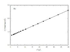
Experimental data is usually plotted as $C_{V}/T$ vs $T^{2}$ since this gives a straight line which looks nice. The intercept with the $C_{V}$ axis tells us the electron contribution. The heat capacity for copper is shown in the figure.

We can get a rough idea of when the phonon and electron contributions to heat capacity are comparable. Equating (3.103) with (3.145), and writing $24\pi^{2}/5\approx 50$ , we have the the two contributions are equal when $T^{2}\sim T_{D}^{3}/50T_{F}$ . Ballpark figures are $T_{D}\sim 10^{2}K$ and $T_{F}\sim 10^{4}K$ which tells us that we have to get down to temperatures of around $1K$ or so to see the electron contribution.

For many metals, the coefficient $\gamma$ of the linear heat capacity is fairly close to the ideal gas value (within, say, 20% or so). Yet the electrons in a metal are far from free: the Coulomb energy from their interations is at least as important as the kinetic energy. So why does the ideal gas approximation work so well? This was explained in the 1950s by Landau and the resulting theory — usually called Landau’s Fermi liquid theory — is the basis for our current understanding of electron systems.

3.6.4 A More Rigorous Approach: The Sommerfeld Expansion

The discussion in Section 3.6.3 uses some approximations but highlights the physics of the low-temperature fermi gas. For completeness, here we present a more rigorous derivation of the low-temperature expansion.

To start, we introduce some new notation for the particle number and energy integrals, (3.135) and (3.136). We write,

	$\displaystyle\frac{N}{V}$	$\displaystyle=$	$\displaystyle\frac{g_{s}}{4\pi^{2}}\left(\frac{2m}{\hbar^{2}}\right)^{3/2}\int% _{0}^{\infty}dE\ \frac{E^{1/2}}{z^{-1}e^{\beta E}+1}$		(3.139)
		$\displaystyle=$	$\displaystyle\frac{g_{s}}{\lambda^{3}}\,f_{3/2}(z)$		(3.139)

and

	$\displaystyle\frac{E}{V}$	$\displaystyle=$	$\displaystyle\frac{g_{s}}{4\pi^{2}}\left(\frac{2m}{\hbar^{2}}\right)^{3/2}\int% _{0}^{\infty}dE\ \frac{E^{3/2}}{z^{-1}e^{\beta E}+1}$		(3.140)
		$\displaystyle=$	$\displaystyle\frac{3}{2}\frac{g_{s}}{\lambda^{3}}k_{B}T\,f_{5/2}(z)$		(3.140)

where $\lambda=\sqrt{2\pi\hbar^{2}/mk_{B}T}$ is the familiar thermal wavelength and the functions $f_{n}(z)$ are the fermionic analogs of $g_{n}$ defined in (3.116),

\displaystyle f_{n}(z)=\frac{1}{\Gamma(n)}\int_{0}^{\infty}dx\ \frac{x^{n-1}}{% z^{-1}e^{x}+1}

(3.141)

where it is useful to recall $\Gamma(3/2)=\sqrt{\pi}/2$ and $\Gamma(5/2)=3\sqrt{\pi}/4$ (which follows, of course, from the property $\Gamma(n+1)=n\Gamma(n)$ ). This function is an example of a polylogarithm and is sometimes written as $Li_{n}(-z)=-f_{n}(z)$ .

Expanding $f_{n}(z)$

We will now derive the large $z$ expansion of $f_{n}(z)$ , sometimes called the Sommerfeld expansion. The derivation is a little long. We begin by splitting the $d x$ integral into two parts,

$\displaystyle\Gamma(n)f_{n}(z)$	$\displaystyle=$	$\displaystyle\int_{0}^{\beta\mu}dx\ \frac{x^{n-1}}{z^{-1}e^{x}+1}+\int_{\beta% \mu}^{\infty}dx\ \frac{x^{n-1}}{z^{-1}e^{x}+1}$
	$\displaystyle=$	$\displaystyle\int_{0}^{\beta\mu}dx\ x^{n-1}\left(1-\frac{1}{1+ze^{-x}}\right)+% \int_{\beta\mu}^{\infty}dx\ \frac{x^{n-1}}{z^{-1}e^{x}+1}$
	$\displaystyle=$	$\displaystyle\frac{(\log z)^{n}}{n}-\int_{0}^{\beta\mu}dx\ \frac{x^{n-1}}{1+ze% ^{-x}}+\int_{\beta\mu}^{\infty}dx\ \frac{x^{n-1}}{z^{-1}e^{x}+1}$

We now make a simple change of variable, $\eta_{1}=\beta\mu-x$ for the first integral and $\eta_{2}=x-\beta\mu$ for the second,

\displaystyle\Gamma(n)f_{n}(z)=\frac{(\log z)^{n}}{n}-\int_{0}^{\beta\mu}d\eta% _{1}\ \frac{(\beta\mu-\eta_{1})^{n-1}}{1+e^{\eta_{1}}}+\int_{0}^{\infty}d\eta_% {2}\ \frac{(\beta\mu+\eta_{2})^{n-1}}{1+e^{\eta_{2}}}

So far we have only massaged the integral into a useful form. We now make use of the approximation $\beta\mu\gg 1$ . Firstly, we note that the first integral has a $e^{\eta_{1}}$ suppression in the denominator. If we replace the upper limit of the integral by $\infty$ , the expression changes by a term of order $e^{-\beta\mu}=z^{-1}$ which is a term we’re willing to neglect. With this approximation, we can combine the two integrals into one,

\displaystyle\Gamma(n)f_{n}(z)=\frac{(\log z)^{n}}{n}+\int_{0}^{\infty}d\eta\ % \frac{(\beta\mu+\eta)^{n-1}-(\beta\mu-\eta)^{n-1}}{1+e^{\eta}}

We now Taylor expand the numerator,

$\displaystyle(\beta\mu+\eta)^{n-1}-(\beta\mu-\eta)^{n-1}$	$\displaystyle=$	$\displaystyle(\beta\mu)^{n-1}\left[(1+\eta/\beta\mu)^{n-1}-(1-\eta/\beta\mu)^{% n-1}\right]$
	$\displaystyle=$	$\displaystyle(\beta\mu)^{n-1}\left[1+(n-1)\frac{\eta}{\beta\mu}+\ldots-1+(n-1)% \frac{\eta}{\beta\mu}+\ldots\right]$
	$\displaystyle=$	$\displaystyle 2(n-1)(\beta\mu)^{n-2}\eta+\ldots$

From which we get

\displaystyle\Gamma(n)f_{n}(z)=\frac{(\log z)^{n}}{n}+2(n-1)(\log z)^{n-2}\int% _{0}^{\infty}d\eta\ \frac{\eta}{e^{\eta}+1}

We’re left with a fairly simple integral.

$\displaystyle\int_{0}^{\infty}\!d\eta\ \frac{\eta}{e^{\eta}+1}$	$\displaystyle=$	$\displaystyle\int_{0}^{\infty}\!d\eta\ \frac{\eta e^{-\eta}}{1+e^{-\eta}}$
	$\displaystyle=$	$\displaystyle\int_{0}^{\infty}\!d\eta\ \eta\sum_{m=1}^{\infty}e^{-m\eta}(-1)^{% m+1}$
	$\displaystyle=$	$\displaystyle\sum_{m=1}^{\infty}\frac{(-1)^{m+1}}{m^{2}}\int_{0}^{\infty}\!du% \ ue^{-u}$

The integral in the last line is very simple: $\int_{0}^{\infty}\!du\ ue^{-u}=1$ . We have only to do the sum. There are a number of ways to manipulate this. We chose to write

	$\displaystyle 1-\frac{1}{2^{2}}+\frac{1}{3^{2}}-\frac{1}{4^{2}}\ldots$	$\displaystyle=$	$\displaystyle\left(1+\frac{1}{2^{2}}+\frac{1}{3^{2}}+\frac{1}{4^{2}}+\ldots% \right)-2\left(\frac{1}{2^{2}}+\frac{1}{4^{2}}+\frac{1}{6^{2}}+\ldots\right)$		(3.142)
		$\displaystyle=$	$\displaystyle\left(1-\frac{2}{2^{2}}\right)\cdot\left(1+\frac{1}{2^{2}}+\frac{% 1}{3^{2}}+\ldots\right)$		(3.142)

This final sum is well known. It is $\sum 1/m^{2}=\zeta(2)=\pi^{2}/6$ . (The original proof of this, by Euler, proceeds by Taylor expanding $\sin x/x$ , writing resulting sum as a product of roots, and then equating the $x^{2}$ term).

After all this work, we finally have the result we want. The low temperature expansion of $f_{n}(z)$ is an expansion in $1/\log z=1/\beta\mu$ ,

\displaystyle f_{n}(z)=\frac{(\log z)^{n}}{\Gamma(n+1)}\left(1+\frac{\pi^{2}}{% 6}\frac{n(n-1)}{(\log z)^{2}}+\ldots\right)

(3.143)

Back to Physics: Heat Capacity of a Fermi Gas Again

The expansion (3.143) is all we need to determine the leading order effects of temperature on the Fermi gas. The number of particles (3.139) can be expressed in terms of the chemical potential as

\displaystyle\frac{N}{V}=\frac{g_{s}}{6\pi^{2}\hbar^{3}}\left(2m\mu\right)^{3/% 2}\left(1+\frac{\pi^{2}}{8}\left(\frac{k_{B}T}{\mu}\right)^{2}+\ldots\right)

(3.144)

But the number of particles determines the Fermi energy through (3.132). For fixed particle number $N$ , we can therefore express the chemical potential at finite temperature in terms of the Fermi energy. After a small amount of algebra, we find

\displaystyle\mu=E_{F}\left(1-\frac{\pi^{2}}{12}\left(\frac{k_{B}T}{E_{F}}% \right)^{2}+\ldots\right)

We see that the chemical potential is a maximum at $T=0$ and decreases at higher $T$ . This is to be expected: recall that by the time we get to the classical gas, the chemical potential must be negative. Moreover, note that the leading order correction is quadratic in temperature rather than linear, in agreement with our earlier claim (3.137).

The energy density can be computed from (3.140) and (3.143). It is

\displaystyle\frac{E}{V}=\frac{g_{s}}{10\pi^{2}\hbar^{3}}(2m)^{3/2}\mu^{5/2}% \left(1+\frac{5\pi^{2}}{8}\left(\frac{k_{B}T}{\mu}\right)^{2}+\ldots\right)

Our real interest is in the heat capacity. However, with fixed particle number $N$ , the chemical potential also varies with temperature at quadratic order. We can solve this problem by dividing by (3.144) to get

\displaystyle\frac{E}{N}=\frac{3E_{F}}{5}\left(1+\frac{5\pi^{2}}{12}\left(% \frac{k_{B}T}{E_{F}}\right)^{2}+\ldots\right)

Now the only thing that depends on temperature on the right-hand side is $T$ itself. From this we learn that the heat capacity of a low temperature Fermi gas is linear in $T$ ,

\displaystyle C_{V}=\left.\frac{\partial{E}}{\partial{T}}\right|_{N,V}=Nk_{B}% \frac{\pi^{2}}{2}\frac{T}{T_{F}}

(3.145)

But we now have the correct coefficient that completes our earlier result (3.138).

3.6.5 White Dwarfs and the Chandrasekhar limit

When stars exhaust their fuel, the temperature $T\rightarrow 0$ and they have to rely on the Pauli exclusion principle to support themselves through the degeneracy pressure (3.134). Such stars supported by electron degeneracy pressure are called white dwarfs. In addition to the kinetic energy $E_{\rm kinetic}$ of fermions given in (3.132) the system has gravitational energy. If we make the further assumption that the density in a star of radius $R$ is uniform, then

\displaystyle E_{\rm grav}=-\frac{3}{5}\frac{G_{N}M^{2}}{R}

where $G_{N}$ is Newton’s constant. In the problem set, you will minimise $E_{\rm grav}+E_{\rm kinetic}$ to find the relationship between the radius and mass of the star,

\displaystyle R\sim M^{-1/3}

This is unusual. Normally if you throw some stuff on a pile, the pile gets bigger. Not so for stars supported by degeneracy pressure. The increased gravitational attraction wins and causes them to shrink.

As the star shrinks, the Fermi energy (3.132) grows. Eventually it becomes comparable to the electron mass $m_{e}$ and our non-relativistic approximation breaks down. We can re-do our calculations using the relativistic formula for the density of states (3.93) (which needs to be multiplied by a factor of 2 to account for the spin degeneracy). In the opposite regime of ultra-relativistic electrons, where $E\gg m_{e}$ , then we can expand the density of states as

\displaystyle g(E)=\frac{V}{\pi^{2}\hbar^{3}c^{3}}\left(E^{2}-\frac{m^{2}c^{4}% }{2}+\ldots\right)

from which we can determine the kinetic energy due to fermions, replacing the non-relativistic result (3.133) by

\displaystyle E_{\rm kinetic}=\frac{V}{\pi^{2}\hbar^{3}c^{3}}\left(\frac{1}{4}% E_{F}^{4}-\frac{m^{2}c^{4}}{4}E_{F}^{2}+\ldots\right)

The Fermi energy can be expressed in terms of the particle number by

\displaystyle N=\frac{V}{\pi^{2}\hbar^{3}c^{3}}\left(\frac{1}{3}E_{F}^{3}-% \frac{m^{2}c^{4}}{2}E_{F}+\ldots\right)

The total energy of the system is then given by,

\displaystyle E_{\rm grav}+E_{F}=\left[\frac{3\hbar c}{4}\left(\frac{9\pi M^{4% }}{4m^{4}_{p}}\right)^{1/3}-\frac{3}{5}G_{N}M^{2}\right]\frac{1}{R}+{\cal O}(R)

where $m_{p}$ is the proton mass (and we’re taking $M=Nm_{p}$ as a good approximation to the full mass of the star). If the term above is positive then the star once again settles into a minimum energy state, where the $1/R$ term balances the term that grows linearly in $R$ . But if the $1/R$ term is negative, we have a problem: the star is unstable to gravitational collapse and will shrink to smaller and smaller values of $R$ . This occurs when the mass exceeds the Chandrasekhar limit, $M>M_{C}$ . Neglecting factors of 2 and $\pi$ , this limit is

\displaystyle M_{C}\sim\left(\frac{\hbar c}{G_{N}}\right)^{3/2}\frac{1}{m_{p}^% {2}}

(3.146)

This is roughly $1.5$ times the mass of the Sun. Stars that exceed this bound will not end their life as white dwarfs. Their collapse may ultimately be stopped by degeneracy pressure of neutrons so that they form a neutron star. Or it may not be stopped at all in which case they form a black hole.

The factor in brackets in (3.146) is an interesting mix of fundamental constants associated to quantum theory, relativity and gravity. In this combination, they define a mass scale called the Planck mass,

\displaystyle M_{pl}^{2}=\frac{\hbar c}{G_{N}}

When energy densities reach the Planck scale, quantum gravity effects are important meaning that we have to think of quantising spacetime itself. We haven’t quite reached this limit in white dwarf stars. (We’re shy by about 25 orders of magnitude or so!). Nonetheless the presence of the Planck scale in the Chandra limit is telling us that both quantum effects and gravitational effects are needed to understand white dwarf stars: the matter is quantum; the gravity is classical.

3.6.6 Pauli Paramagnetism

“With heavy heart, I have decided that Fermi-Dirac, not Einstein, is the correct statistics, and I have decided to write a short note on paramagnetism”

Wolfgang Pauli, in a letter to Schrödinger, reluctantly admitting that electrons are fermions

We now describe a gas of electrons in a background magnetic field $\vec{B}$ . There are two effects that are important: the Lorentz force $\vec{v}\times B$ on the motion of electrons and the coupling of the electron spin to the magnetic field. We first discuss the spin coupling and postpone the Lorentz force for the next section.

An electron can have two spin states, “up” and “down”. We’ll denote the spin state by a discrete label: $s=1$ for spin up; $s=-1$ for spin down. In a background magnetic field $\vec{B}$ , the kinetic energy picks up an extra term

\displaystyle E_{\rm spin}=\mu_{B}Bs

(3.147)

where $\mu_{B}=|e|\hbar/2m$ is the Bohr magneton. (It has nothing to do with the chemical potential. Do not confuse them!)

Since spin up and spin down electrons have different energies, their occupation numbers differ. Equation (3.139) is now replaced by

	$\displaystyle\frac{N_{\uparrow}}{V}$	$\displaystyle=$	$\displaystyle\frac{1}{4\pi^{2}}\left(\frac{2m}{\hbar^{2}}\right)^{3/2}\int_{0}% ^{\infty}dE\ \frac{E^{1/2}}{e^{\beta(E+\mu_{B}B-\mu)}+1}=\frac{1}{\lambda^{3}}% f_{3/2}(ze^{-\beta\mu_{B}B})$
	$\displaystyle\frac{N_{\downarrow}}{V}$	$\displaystyle=$	$\displaystyle\frac{1}{4\pi^{2}}\left(\frac{2m}{\hbar^{2}}\right)^{3/2}\int_{0}% ^{\infty}dE\ \frac{E^{1/2}}{e^{\beta(E-\mu_{B}B-\mu)}+1}=\frac{1}{\lambda^{3}}% f_{3/2}(ze^{+\beta\mu_{B}B})$

Our interest is in computing the magnetization, which is a measure of how the energy of the system responds to a magnetic field,

\displaystyle M=-\frac{\partial{E}}{\partial{B}}

(3.148)

Since each spin has energy (3.147), the magnetization is simply the difference in the in the number of up spins and down spins,

\displaystyle M=-\mu_{B}(N_{\uparrow}-N_{\downarrow})=-\frac{\mu_{B}V}{\lambda% ^{3}}\left[f_{3/2}(ze^{-\beta\mu_{B}B})-f_{3/2}(ze^{\beta\mu_{B}B})\right]

At high temperatures, and suitably low magnetic fields, we can approximate $f_{3/2}(z)\approx z$ as $z\rightarrow 0$ , so that

\displaystyle M\approx\frac{2\mu_{B}Vz}{\lambda^{3}}\sinh(\beta\mu_{B}B)

We can eliminate the factor of $z$ in favour of the particle number,

\displaystyle N=N_{\uparrow}+N_{\downarrow}\approx\frac{2Vz}{\lambda^{3}}\cosh% (\beta\mu_{B}B)

From which we can determine the high temperature magnetization,

\displaystyle M\approx\mu_{B}N\tanh(\beta\mu_{B}B)

This is the same result that you computed in the first problem sheet using the simple two-state model. We see that, once again, at high temperatures the quantum statistics are irrelevant. The magnetic susceptibility is a measure of how easy it is to magnetise a substance. It is defined as

\displaystyle\chi\equiv\frac{\partial{M}}{\partial{B}}

(3.149)

Evaluating $\chi$ in the limit of vanishing magnetic field, we find that the magnetization is inversely proportional to the temperature,

\displaystyle\chi(B=0)=\frac{N\mu_{B}^{2}}{k_{B}T}

This $1/T$ behaviour is known as Curie’s law. (Pierre, not Marie).

The above results hold in the high temperature limit. In contrast, at low temperatures the effects of the Fermi surface become important. We need only keep the leading order term in (3.143) to find

\displaystyle M\approx\frac{\mu_{B}V}{6\pi^{2}}\left(\frac{2m}{\hbar^{2}}% \right)^{3/2}\left[(E_{F}+\mu_{B}B)^{3/2}-(E_{F}-\mu_{B}B)^{3/2}\right]\approx% \frac{\mu_{B}^{2}V}{2\pi^{2}}\left(\frac{2m}{\hbar^{2}}\right)^{3/2}E_{F}^{1/2}B

where we’re written the final result in the limit $\mu_{B}B\ll E_{F}$ and expanded to linear order in $B$ . We could again replace some of the factors for the electron number $N$ . However, we can emphasise the relevant physics slightly better if we write the result above in terms of the density of states (3.108). Including the factor of 2 for spin degeneracy, we have

\displaystyle M\approx\mu_{B}^{2}g(E_{F})B

(3.150)

We see that at low temperatures, the magnetic susceptibility no longer obeys Curie’s law, but saturates to a constant

\displaystyle\chi\equiv\frac{\partial{M}}{\partial{B}}=\mu_{B}^{2}g(E_{F})

What’s happening here is that most electrons are embedded deep within the Fermi surface and the Pauli exclusion principle forbids them from flipping their spins in response to a magnetic field. Only those electrons that sit on the Fermi surface itself — all $g(E_{F})$ of them — have the luxury to save energy by aligning their spins with the magnetic field.

Notice that $\chi>0$ . Such materials are called paramagnetic: in the presence of a magnetic field, the magnetism increases. Materials that are paramagnetic are attracted to applied magnetic fields. The effect described above is known as Pauli paramagnetism.

3.6.7 Landau Diamagnetism

For charged fermions, such as electrons, there is a second consequence of placing them in a magnetic field: they move in circles. The Hamiltonian describing a particle of charge $-e$ in a magnetic field $\vec{B}=\nabla\times\vec{A}$ is,

\displaystyle H=\frac{1}{2m}\left(\vec{p}+e\vec{A}(\vec{r})\right)^{2}

This has an immediate consequence: a magnetic field cannot affect the statistical physics of a classical gas! This follows simply from substituting the above Hamiltonian into the classical partition function (2.49). A simple shift of variables, $\vec{p}^{\prime}=\vec{p}+e\vec{A}$ shows that the classical partition function does not depend on $\vec{B}$ . This result (which was also mentioned in a slightly different way in the Classical Dynamics course) is known as the Bohr-van Leeuwen theorem: it states that there can be no classical magnetism.

Let’s see how quantum effects change this conclusion. Our first goal is to understand the one-particle states for an electron in a constant background magnetic field. This is a problem that you will also solve in the Applications of Quantum Mechanics course. It is the problem of Landau levels.

Landau Levels

We will consider an electron moving in a constant magnetic field pointing in the $\hat{z}$ direction: $\vec{B}=(0,0,B)$ . There are many different ways to pick $\vec{A}$ such that $\vec{B}=\nabla\times\vec{A}$ gives the right magnetic field. These are known as gauge choices. Each choice will give rise to the same physics but, usually, very different equations in the intervening steps. Here we make the following gauge choice,

\displaystyle\vec{A}=(-By,0,0)

(3.151)

Let’s place our particle in a cubic box with sides of length $L$ . Solutions to the Schrödinger equation $\hat{H}\psi=E\psi$ are simply plane waves in the $x$ and $z$ directions,

\displaystyle\psi(\vec{r})=e^{i(k_{x}x+k_{z}z)}f(y)

But the wavefunction $f(y)$ must satisfy,

\displaystyle\left[-\frac{\hbar^{2}}{2m}\frac{\partial^{2}}{\partial y^{2}}+% \frac{1}{2m}\left(\hbar k_{x}-eBy\right)^{2}\right]f(y)=E^{\prime}f(y)

(3.152)

But this is a familiar equation! If we define the cyclotron frequency,

\displaystyle\omega_{c}=\frac{eB}{m}

Then we can rewrite (3.152) as

\displaystyle\left[-\frac{\hbar^{2}}{2m}\frac{\partial^{2}}{\partial y^{2}}+% \frac{1}{2}m\omega_{c}^{2}\left(y-y_{0}\right)^{2}\right]f(y)=E^{\prime}f(y)

where $y_{0}=\hbar k_{x}/eB$ . This is simply the Schrödinger equation for a harmonic oscillator, jiggling with frequency $\omega_{c}$ and situated at position $y_{0}$ .

One might wonder why the harmonic oscillator appeared. The cyclotron frequency $\omega_{c}$ is the frequency at which electrons undergo classical Larmor orbits, so that kind of makes sense. But why have these become harmonic oscillators sitting at positions $y_{0}$ which depend on $k_{x}$ ? The answer is that there is no deep meaning to this at all! it is merely an artefact of our gauge choice (3.151). Had we picked a different $\vec{A}$ giving rise to the same $\vec{B}$ , we would find ourselves trying to answer a different question! The lesson here is that when dealing with gauge potentials, the intermediate steps of a calculation do not always have physical meaning. Only the end result is important. Let’s see what this is. The energy of the particle is

\displaystyle E=E^{\prime}+\frac{\hbar^{2}k_{z}^{2}}{2m}

where $E^{\prime}$ is the energy of the harmonic oscillator,

\displaystyle E^{\prime}=\left(n+\frac{1}{2}\right)\hbar\omega_{c}\ \ \ \ \ \ % n\in{\bf Z}

These discrete energy levels are known as Landau levels. They are highly degenerate. To see this, note that $k_{x}$ is quantized in unit of $\Delta k_{x}=2\pi/L$ . This means that we can have a harmonic oscillator located every $\Delta y_{0}=2\pi\hbar/eBL$ . The number of such oscillators that we can fit into the box of size $L$ is $L/\Delta y_{0}$ . This is the degeneracy of each level,

\displaystyle\frac{eBL^{2}}{2\pi\hbar}\equiv\frac{\Phi}{\Phi_{0}}

where $\Phi=L^{2}B$ is the total flux through the system and $\Phi_{0}=2\pi\hbar/{e}$ is known as the flux quantum. (Note that the result above does not include a factor of 2 for the spin degeneracy of the electron).

Back to the Diamagnetic Story

We can now compute the grand partition function for non-interacting electrons in a magnetic field. Including the factor of 2 from electron spin, we have

\displaystyle\log{\cal Z}=\frac{L}{2\pi}\int dk_{z}\sum_{n=0}^{\infty}\frac{2L% ^{2}B}{\Phi_{0}}\log\left[1+z\exp\left(-\frac{\beta\hbar^{2}k_{z}^{2}}{2m}-% \beta\hbar\omega_{c}(n+1/2)\right)\right]

To perform the sum, we use the Euler summation formula which states that for any function $h(x)$ ,

\displaystyle\sum_{n=0}^{\infty}h(n+1/2)=\int_{0}^{\infty}h(x)dx+\frac{1}{24}h% ^{\prime}(0)+\ldots

We’ll apply the Euler summation formula to the function,

\displaystyle h(x)=\int dk_{z}\log\left[1+\exp\left(-\frac{\beta\hbar^{2}k_{z}% ^{2}}{2m}+\beta x\right)\right]

So the grand partition function becomes

$\displaystyle\log{\cal Z}$	$\displaystyle=$	$\displaystyle\frac{VB}{\pi\Phi_{0}}\sum_{n=0}^{\infty}h(\mu-\hbar\omega_{c}(n+% 1/2))$	(3.153)
	$\displaystyle=$	$\displaystyle\frac{VB}{\pi\Phi_{0}}\int_{0}^{\infty}h(\mu-\hbar\omega_{c}x)\,% dx-\frac{VB}{\pi\Phi_{0}}\frac{\hbar\omega_{c}}{24}\frac{dh(\mu)}{d\mu}+\ldots$
	$\displaystyle=$	$\displaystyle\frac{Vm}{2\pi^{2}\hbar^{2}}\left[\int_{-\infty}^{\mu}h(y)\,dy-% \frac{(\hbar\omega_{c})^{2}}{24}\int_{-\infty}^{+\infty}dk\ \frac{\beta}{e^{% \beta(\hbar^{2}k^{2}/2m-\mu)}+1}\right]+\ldots$

The first term above does not depend on $B$ . In fact it is simply a rather perverse way of writing the partition function of a Fermi gas when $B=0$ . However, our interest here is in the magnetization which is again defined as (3.148). In the grand canonical ensemble, this is simply

\displaystyle M=\frac{1}{\beta}\frac{\partial{\log{\cal Z}}}{\partial{B}}

The second term in (3.153) is proportional to $B^{2}$ (which is hiding in the $\omega_{c}^{2}$ term). Higher order terms in the Euler summation formula will carry higher powers of $B$ and, for small $B$ , the expression above will suffice.

At $T=0$ , the integrand is simply $1$ for $|k|<k_{F}$ and zero otherwise. To compare to Pauli paramagnetism, we express the final result in terms of the Bohr magneton $\mu_{B}=|e|\hbar/2mc$ . We find

\displaystyle M=-\frac{\mu_{B}^{2}}{3}g(E_{F})B

This is comparable to the Pauli contribution (3.150). But it has opposite sign. Substances whose magnetization is opposite to the magnetic field are called diamagnetic: they are repelled by applied magnetic fields. The effect that we have derived above is known as Landau diamagnetism.