2.7  GIS effects

The GIS spectra have various effects that must be carefully considered before starting any data analysis. Some effects are typical of any MCP detector, and are

electronic dead times

short term gain depression

long term gain depression.

The GIS operates by sending a continuous stream of event positions to the Command and Data-Handling System (CDHS). The various electronic dead-times are such that any events occurring within about 10 ms of each other will be rejected, and higher rates will render the data meaningless.

Short term gain depression occurs when count rates per pixel are above 40. In this situation, the MCP cannot re-charge fast enough to provide full gain for every event, and the data are not usable.

Long term gain depression is an ageing effect, a reduction in detector sensitivity over a long time interval due to continued illumination. The applied high voltage can be increased to compensate for the decrease in the MCP gain with time. However, the gain depression will be greatest at the position of the brightest lines so a wavelength-dependent effect will remain.

2.7.1  Fixed patterning and line profiles

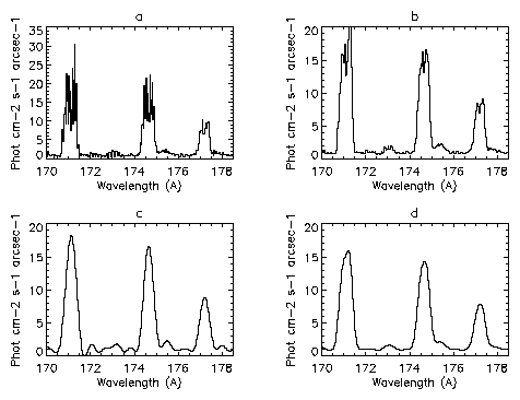
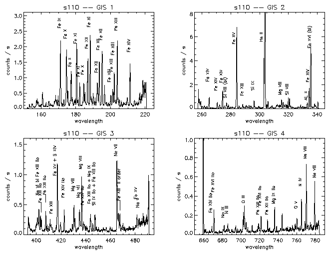
The profiles of the GIS lines are predominantly instrumental. They are corrupted by the superposition of a spiky effect on the whole spectrum, referred to as fixed patterning. Counts falling near the boundary of a pixel can be shifted to neighbouring pixels, producing narrow spikes and troughs in the profiles of the emission lines. Weaker lines can appear swamped by this effect.

Figure 3a shows a portion of the GIS 1 spectrum, as an example. It is not only impossible to define a line profile, but even hard to recognise the presence of weak lines. Fixed patterning should not alter the total counts recorded in an emission line; it merely displaces some of them.

Figure 3: Effects of different smoothing procedures applied to a portion of the GIS 1 active region spectrum. a: original spectrum; b: box-smoothed spectrum; c: Fourier-filtered spectrum; d: Gaussian-convolved spectrum.

2.7.2  Ghosts

For some lines, the cluster of photon events will tend to spread across to the neighbouring arms of the spiral. This happens when the width of the spiral is broadened by electronic noise. This effect tends to occur only in those regions where the spiral arms are close together, and can lead to spreading to one of the adjacent arms (or both).

Figure 4: [from MSSL user guide] A GIS 1 spectrum output from ghost_plot_one, (top-top) theoretical quiet sun spectrum, (top-middle) left shifted spectrum, (top-bottom) right shifted spectrum. (Bottom) Spectrum to be de-ghosted, with likely ghosting regions shaded.

Figure 5: A GIS 1 ghosting region.

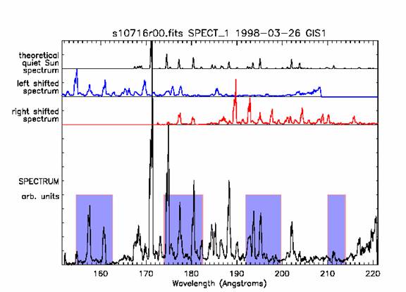
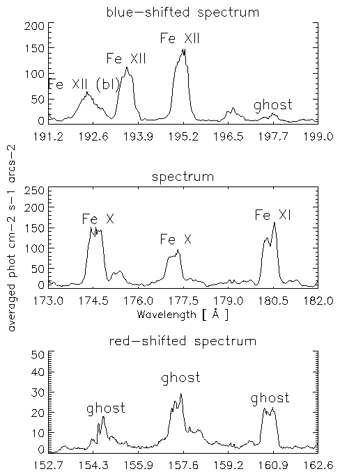
Now, once a set of LUTs is applied to the data on-board, i.e. a particular spiral pattern is assumed appropriate for the data, the original information is lost. In terms of counts versus wavelength, this means that a portion of the counts belonging to a line can be shifted into different parts of the telemetered spectrum, giving rise to spurious spectral lines if they fall in a spectral region void of lines, or providing extra intensity to already existing spectral lines. Henceforth we will refer to a spectral line whose intensity is enhanced in this way as ghosted (or contaminated) line, while the lines whose counts have been partially shifted toward other regions of the spectrum will be referred to as ghosting (or parent) lines. The counts shifted by this effect will be called ghosts, while the process will be called simply ghosting.

Since the spreading can only occur toward one or the other side of a spiral arm, each line can generate no more than two ghosts. When the spreading occurs toward the outer arm, a ghost is created at a lower wavelength, in the so-called red-shifted spectrum. Conversely, when part of the counts of a line are read into the inner arm, a ghost is created at a higher wavelength (in the so-called blue-shifted spectrum). Note that the definitions of red-shifted and blue-shifted GIS spectra do not have any relation to physical blue- or red-shifts, nor these spectra are simply `shifted' (in fact, they are compressed or expanded in the wavelength scale).

For each application of a given set of LUTs, ghosts will appear in the same positions. Once the applied LUTs are known, it is therefore possible to deduce which regions of the spectrum are unlikely to be affected by them, and to predict where ghosts might appear. It is therefore theoretically possible to deghost (or reconstruct) the spectra, i.e. add to each line the intensity lost by the creation of a ghost.

Unfortunately, the situation is quite complex, for many reasons.

• First, different LUTs (i.e. spectra with different GSET_ID) produce different ghosting.
• Then, there are no general rules that can be applied to deghost the spectra. Only when a ghost appears in a region of the spectrum free of lines, is it possible to reconstruct the depleted line from which it came.
• Usually it is very difficult to distinguish between the ghost and any real lines with which it is blended.

Figure 6: The first light GIS spectra of a coronal hole (s90)

Figure 7: One of the first series of GIS spectra of a quiet sun (s132) region.

Figure 8: The first light GIS spectra of an active region (s110).