4.3  NIS and GIS sensitivities

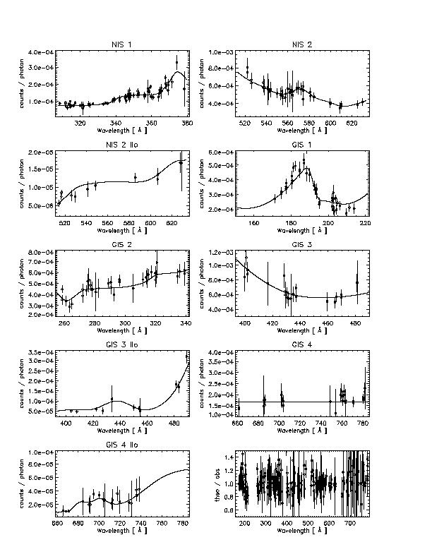
Figure 22: The CDS NIS and GIS sensitivities (solid lines), first and second order, as derived from pre-recovery observations. The absolute sensitivities derived from all the line ratios used are superimposed. The bottom right plot shows the ratio of the theoretical vs. the observed line intensities for all the line used.

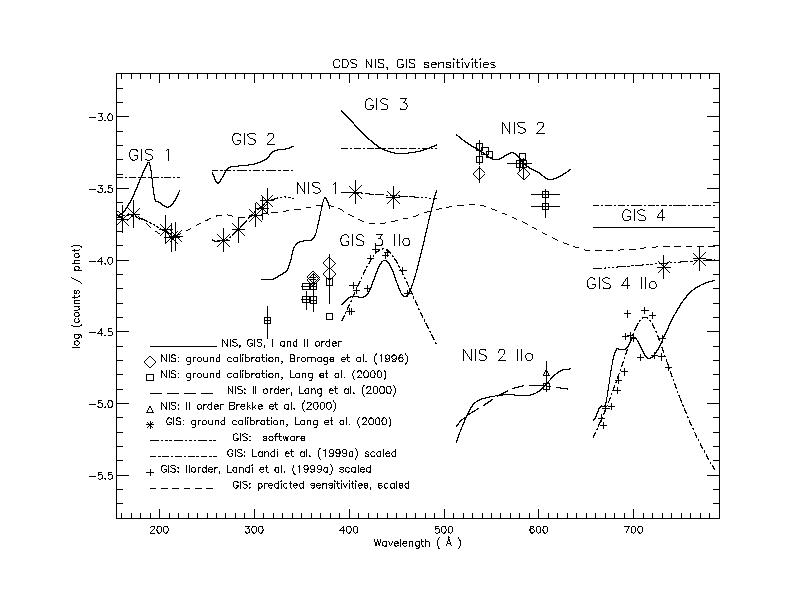
Figure 23: The CDS NIS and GIS first and second order sensitivities proposed here (solid lines). All the pre-launch NIS and GIS measurements are also displayed. The overall GIS predicted efficiency, as a function of wavelength, is plotted with a dashed line (arbitrary scale). For the NIS 2 second order, the value found by Brekke et al. (2000) is also shown. For the GIS, the sensitivities derived by Landi et al., (1999a) for the first and second orders are also displayed (absolute values scaled by a factor of 2). For the GIS 3 and 4 second orders, the points used by Landi et al. (1999a) to derive the curves are also displayed (crosses), to show that those data are broadly consistent with the curves presented here.

The main features of the calibration presented here, compared to the previous studies are:

• Much increased sensitivities in NIS 1 and in all the GIS channels, compared to the pre-launch values. For the NIS 1 case, the factor is about 2 (1.9 at 317 Å and 2.2 at 362 Å), while for the GIS case the factors are more variable (1.45 at 206 Å, GIS 1; 2.8 at 283 Å, GIS 2; 2.9 at 406 Å, GIS 3; 1.9 at 732 Å, GIS 4).
• Good agreement for NIS 1 with other in-flight studies.
• For GIS, it is interesting to note that the calibration proposed here would explain the discrepancies that were found when the SUMER and the GIS calibrations were compared in-flight at 770 Å, and where a factor of 2 was also found (Pauluhn, 2001, priv. comm.).
• Excellent agreement (within few percent) of the second order NIS 2 sensitivity at 608 Å (He II 304 Å line, 1.36 × 10^-5) compared to the only pre-launch measurement by Lang et al. (2000; 1.32 ±0.11 × 10^-5). The measurement of Brekke et al. (2000) is about 20% higher (1.64 ±0.12 × 10^-5), while the SERTS-97 flight has provided a value of 1.68 ±0.25 × 10^-5 (R. Thomas, priv. comm.).

  Some differences with the predicted second order sensitivities at the other wavelengths are found.

• The wavelength variations of the sensitivities, within each GIS channel, can be regarded as consistent with the few pre-launch GIS measurements, except for GIS 2 where a steeper wavelength dependence was measured on the ground.

  Note, however, that the absolute values of the predicted sensitivities are about a factor of 10 higher than the values presented here.

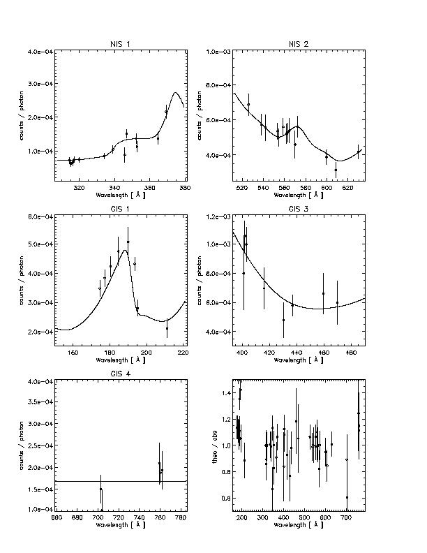
4.3.1  Post-recovery sensitivities

Figure 24: The CDS NIS and GIS pre-recovery sensitivities as in Fig. 23, with the values derived from the post-recovery observations of May 1999. The bottom right plot shows the ratio of the theoretical vs. the observed line intensities.

No significant changes in the calibration appear to be present from a single dataset (Del Zanna et al. 2001). However, there are many indications that the sensitivities have changed, in particular the NIS 1 one. See the book on the SOHO radiometric calibration.