1 From Spins to Fields
The ideas that we will introduce in these lectures have wide applicability across many areas of physics. However, we will spend much of these lectures studying just a single example. This example is known as the Ising model and it provides a particularly simple model of a magnet. Despite its simplicity, the Ising model already contains many of the concepts that will keep us occupied for the rest of the course. Having understood the Ising model in some detail, we see how these ideas play out in many other phases of matter in Section 4.
1.1 The Ising Model
The Ising model is easy to state, yet hard to solve. We have a lattice in spatial dimensions, containing sites. On each lattice site , there lives a discrete variable which can take one of two states: or .
It is useful to refer to these states as spins, with corresponding to spin up, and to spin down. However, we won’t be using any machinery from quantum mechanics: there are no non-commuting operators, nor quantum superpositions of states. In this sense, the Ising model, while discrete, is purely classical.
The collection of spins has energy
| (1.1) |
The first term arises due to an external magnetic field, that we impose on the system. It has the effect that, for , the spins want to be up because that will lower their energy. (Properly this should be the magnetising field , but we’re using to avoid confusion with the Hamiltonian. There is also a factor of the magnetic moment that we’ve absorbed into .)
With the first term alone, the individual spins don’t talk to each other and the model is easy to solve. It is the second term that makes life more interesting. This is an interaction between neighbouring spins. The notation means that we sum over all “nearest neighbour” pairs in the lattice. The number of such pairs depends both on the dimension and the type of lattice.
If , neighbouring spins prefer to be aligned ( or ). In the context of magnetism, such a system is called a ferromagnet. If , the spins want to anti-align (). This is an anti-ferromagnet. In the following, we choose although, for our purposes, the differences are minor.
(For what it’s worth, the anti-ferromagnetic case, with , becomes more subtle on certain lattices where it’s not possible to arrange the spins so that they are opposite to all their neighbours. A 2d triangular lattice provides a simple example. The resulting physics is interesting and is known as (geometrical) frustration. We will not discuss it here.)
We are interested in the physics of the Ising model at a finite temperature . We can already get some intuition for what will happen. The interaction energy encourages the spins to align in the same way. The magnetic field encourages the spins to align in a particular way. Meanwhile, the temperature encourages the spins to ignore both the interactions and magnetic field because, at finite temperature, energy is no longer at a premium. Instead, entropy becomes more important. Since there are many more random configurations than aligned configurations, the temperature will tend to mess up the nice ordered states that the interactions and magnetic field have so carefully prepared. Already we can see that, like any good story, we’re starting with a healthy dose of narrative tension between our main characters.
In the canonical ensemble, the probability of sitting in a configuration of spins is given by
| (1.2) |
where and the normalisation factor is called the partition function, and is given by
| (1.3) |
The beauty of statistical mechanics is that even though is first introduced as an innocuous normalisation factor, it actually contains everything we want to known about the system. If we’re able to perform the sum to compute , we can extract any information we want11 1 The basic machinery of partition functions was described in the first course on Statistical Physics.. For example, the interplay between energy and entropy is captured by the thermodynamic free energy
| (1.4) |
As the notation shows, this is a function of thermodynamic variables, and . (We don’t usually add the subscript “thermo” to the free energy but for much of these lectures we’ll be working with a more refined version of the free energy which we’ll shortly introduce.)
Of particular interest to us will be the average spin of the configuration, which we refer to as the equilibrium magnetization.
| (1.5) |
This takes values is the range . From our discussion above, we would expect that, for , at low temperatures where the spins are ordered, and at high temperatures where the spins are arranged randomly. We’d like to make this intuition more precise. Using the probability (1.2), it is straightforward to check that the magnetisation can be written as
| (1.6) |
Taking further derivatives allows us to compute higher moments of the distribution, and so learn about fluctuations around the average. We will see this in action later in these lectures.
Our task is now clear: we should compute the sum (1.3). This is easier said than done. It turns out that the sum is straightforward in a dimensional lattice, and you will do this on an example sheet. An exact solution also exists in when , originally due to Onsager. It is not straightforward. In higher dimensions, no exact solutions are available, although various expansions and tricks have been invented to manipulate the sum (1.3) to extract some interesting information.
In these lectures, we will not attempt to directly sum the microscopic spins in the partition function. Instead, we will rephrase the question. We will massage the partition function into a somewhat different form, one that has much broader application.
1.1.1 The Effective Free Energy
The key idea was explained in the introduction: Nature is organised by scale. The energy of the Ising model (1.1) provides the microscopic description of our system in terms of individual spins. Computing the partition function exactly gives us a macroscopic description of the system in terms of thermodynamic variables like temperature and magnetic field . What we’re looking for is something in between.
We’re going to get to this “something in between” in two steps: we’ll do something rather crude here, and then do a better job in Section 1.3. For our crude attempt, we rewrite the partition function (1.3) in the following manner:
| (1.7) |
where the notation means all configurations of spins such that . In other words, we first sum over all configurations with fixed average magnetisation , and subsequently sum over all possible .
Note that we’re using here in a subtly different way to the original definition (1.5). In the sum (1.7), the magnetisation refers to the average magnetisation of a given configuration and can take any value. In contrast, in (1.5) we are talking about the equilibrium value of magnetisation, averaged over all configurations in the canonical ensemble. We will see shortly how to find this equilibrium value.
The average magnetisation lies in the range . Strictly speaking, this takes only discrete values, quantised in units of . However, we are ultimately interested in the limit of large , so we don’t lose anything by writing this as an integral,
| (1.8) |
where the factor of is the (inverse) width between the allowed values. Such overall coefficients in the partition function are unimportant for the physics, and we will not be careful in keeping them below.
This way of writing things has allowed us to define something new: an effective free energy, , which depends on the magnetisation of the system, in addition to both and . This goes beyond the usual, thermodynamic idea of free energy given in (1.4) which is defined only in equilibrium, where the magnetisation takes a specific value, determined by (1.6).
Note that (1.8) looks very much like a standard path integral, with playing the role of the energy for . But there is a difference because, unlike in the microscopic theory, can depend on temperature. This means that the dependence in the exponent can be more complicated than we’re used to. We’ll see this explicitly below.
The effective free energy contains more information than the thermodynamic free energy . In particular, can tell us the correct, equilibrium value of the magnetisation . To see this, we define the free energy per unit spin,
Our partition function becomes
Here is a very large number (think ) while . Integrals of this kind are very well approximated by the value of which minimises , an approximation known as the saddle point or steepest descent,
The minimum is the equilibrium value of the magnetisation that we previously computed in (1.6). Substituting this into the the partition function, we have
| (1.9) |
In this way, we can reconstruct from knowledge of .
1.1.2 Mean Field Theory
To proceed, we want to find a way to compute , defined in (1.7). But this is tantamount to performing the sum in the path integral and, as we stressed above, this is not easy. We need to find another way.
We will use a method called the mean field approximation. Here the word “approximation” is somewhat generous; a better name would be the mean field “guess” since there is little justification for what we’re about to do. Instead, the purpose is to provide a starting point for our discussion. Not all the consequences that we derive from this guess will be accurate, but as the lectures progress we’ll get a better understanding about what we can trust, what we can’t, and how to do better.
We wish to sum over configurations with . We can get an estimate for the energy of such configurations by replacing each spin s in (1.1) with its expectation (i.e. mean) value ,
| (1.10) |
Here denotes the number of nearest neighbours of each spin. For example, in a lattice has ; in , a square lattice has . A square lattice in dimensions has . The factor or is there because is a sum over pairs rather than a sum of individual sites.
Among other things, this means that we’re assuming (falsely!) that the energy depends only on the magnetisation of a configuration, rather than any more finely grained details. The sole reason for doing this is that it makes the resulting sum over configurations very easy to do: we simply need to count the number of configurations with magnetisation . A configuration with up spins and down spins has magnetisation
The number of such configurations is
and we can use Stirlings formula to evaluate
In our mean field approximation, the effective free energy defined in (1.7) is then given by
Substituting the energy (1.10), and taking logs of both sides, we find ourselves with the following expression:
From this, we can compute the equilibrium value for . As explained above, this occurs at the minimum
A little algebra shows us that the equilibrium magnetisation obeys the self-consistency condition
| (1.11) |
There’s a nice intuition behind this equation. It can be derived by assuming that each spin experiences an effective magnetic field given by , which includes an extra contribution from the spins around it. In this way, the tricky interactions in the Ising model have been replaced by an averaged effective field . This is sometimes called the mean field and gives its name to this technique.
There are a number of ways forward at this point. We could, for example, analyse the properties of the Ising model by looking at solutions to the self-consistency condition (1.11); this was the strategy taken in the Statistical Physics lectures. However, instead we’re going to focus on the free energy , since this will prove to be the more useful tool moving forward.
1.2 Landau Approach to Phase Transitions
A phase transition occurs when some quantity changes in a discontinuous fashion. For us, this quantity is which, as we will see, will exhibit non-analytic behaviour as we vary different parameters.
Landau theory is a simple, yet effective way to understand the qualitative manner in which these phase transitions occur. It is based on two ideas: the free energy, and symmetry. Here we will apply Landau’s theory to the Ising model, focussing first on the free energy. We will comment on the role of symmetry at the end of this section, although the full power of this idea will only become apparent in Section 4 where we describe a whole raft of further examples.
In the previous section, we introduced the effective free energy , which is a function of the magnetisation . This kind of object is the starting point for Landau’s theory. In this context, the magnetisation is known as an order parameter. Using the mean field approximation, we computed this to be
Landau’s approach focuses on situations where the order parameter is small. Here we can Taylor expand,
| (1.12) |
As we’ve seen above, the preferred value of is simply the minimum of . The idea of Landau theory is simply to observe how the function , and in particular its minima, change as we vary different parameters. Crucially, the story is rather different depending on whether or . We will deal with each of these in turn.
|
|
1.2.1 : A Continuous Phase Transitions
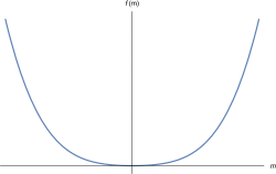
Let’s first consider the situation with vanishing magnetic field, , so that there is no term in (1.12) that is linear in . Since our interest lies in the dependence of , we won’t lose anything if we drop the constant term. We’re left with the free energy
| (1.13) |
The behaviour of the free energy depends on whether the quadratic term is positive or negative. To distinguish between these two, we define the critical temperature
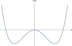
The free energy is sketched in the case where (on the left) and (on the right). We see that at high temperatures, the magnetisation vanishes at the minimum: . This is in agreement with our expectation that temperature will randomise the spins. However, as the temperature is reduced below , the point becomes a maximum of the free energy and the minima now lie at which, if we chose to truncate the free energy (1.13) at order , is given by
| (1.14) |

This form is valid only when is close to , so that is small and higher order terms can be ignored. As the temperature is lowered further, the minimum grows. We’re then obliged to turn to the full form of the free energy which, among other things, knows that the magnetisation lies in the range .
The upshot is that as we vary the temperature, the magnetisation takes the form shown on the right. This is perhaps somewhat surprising. Usually in physics, things turn on gradually. But here the magnetisation turns off abruptly at , and remains zero for all higher temperatures. This kind of sharp change is characteristic of a phase transition. When , we say that the system sits in the disordered phase; when , it is in the ordered phase.
The magnetisation itself is continuous and, for this reason, it is referred to as a continuous phase transition or, sometimes, a second order phase transition.
As an aside: phase transitions can be classified by looking at the thermodynamic free energy and taking derivatives with respect to some thermodynamic variable, like . If the discontinuity first shows up in the derivative, it is said to be an order phase transition. However, in practice we very rarely have to deal with anything other than first order transitions (which we will see below) and second order transitions. In the present case, we’ll see shortly that the heat capacity is discontinuous, confirming that it is indeed a second order transition.
The essence of a phase transition is that some quantity is discontinuous. Yet, this should make us nervous. In principle, everything is determined by the partition function , defined in (1.3), which is a sum of smooth, analytic functions. How is it possible, then, to get the kind of non-analytic behaviour characteristic of a phase transition? The loophole is that is only necessarily analytic if the sum is finite. But there is no such guarantee that it remains analytic when the number of lattice sites . This means that genuine, discontinuous phase transitions only occur in infinite systems. In reality, we have around atoms. This gives rise to functions which are, strictly speaking, smooth, but which change so rapidly that they act, to all intents and purposes, as if they were discontinuous.
These kind of subtleties are brushed under the carpet in the mean field approach that we’re taking here. However, it’s worth pointing out that the free energy, is an analytic function which, when Taylor expanded, gives terms with integer powers of . Nonetheless, the minima of behave in a non-analytic fashion.
For future purposes, it will be useful to see how the heat capacity changes as we approach . In the canonical ensemble, the average energy is given by . From this, we find that we can write the heat capacity as
| (1.15) |
To proceed, we need to compute the partition function , by evaluating at the minimum value as in (1.9). When , this is simple: we have and (still neglecting the constant term which doesn’t contribute to the heat capacity). In contrast, when the minimum lies at given in (1.14), and the free energy is .

Now we simply need to differentiate to get the heat capacity, . The leading contribution as comes from differentiating the piece, rather than the piece. We have
| (1.16) |
We learn that the heat capacity jumps discontinuously. The part of the heat capacity that comes from differentiating terms is often called the singular piece. We’ll be seeing more of this down the line.
Spontaneous Symmetry Breaking
There is one further aspect of the continuous phase transition that is worth highlighting. The free energy (1.13) is invariant under the symmetry . This is no coincidence: it follows because our microscopic definition of the Ising model (1.1) also enjoys this symmetry when .
However, below , the system must pick one of the two ground states or . Whichever choice it makes breaks the symmetry. When a symmetry of a system is not respected by the ground state we say that the symmetry is spontaneously broken. This will become an important theme for us as we move through the course. It is also an idea which plays an important role in particle physics .
Strictly speaking, spontaneous symmetry breaking can only occur in infinite systems, with the magnetisation defined by taking the limit
It’s important that we take the limit , before we take the limit . If we do it the other way round, we find as for any finite .
|
|
1.2.2 : First Order Phase Transitions
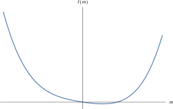
Let’s now study what happens when . Once again, we ignore the constant term in the free energy (1.12). We’re left with the free energy
| (1.17) |
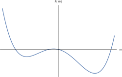
There are again two, qualitatively different forms of this function at low and high temperatures, shown in the figures above for .
At low temperatures there are two minima, but one is always lower than the other. The global minima is the true ground state of the system. The other minima is a meta-stable state. The system can exit the meta-stable state by fluctuating up, and over the energy barrier separating it from the ground state, and so has a finite lifetime. As we increase the temperature, there is a temperature (which depends on ) beyond which the meta-stable state disappears. This temperature is referred to as the spinodal point. It will not play any further role in these lectures.
For us, the most important issue is that the ground state of the system – the global minimum of – does not qualitatively change as we vary the temperature. At high temperatures, the magnetisation asymptotes smoothly to zero as

At low temperatures, the magnetization again asymptotes to the state which minimises the energy. Except this time, there is no ambiguity as to whether the system chooses or . This is entirely determined by the sign of the magnetic field . A sketch of the magnetisation as a function of temperature is shown on the right. The upshot is that, for , there is no phase transition as a function of the temperature.
However, we do not have to look to hard to find a phase transition: we just need to move along a different path in the phase diagram. Suppose that we keep fixed at a value below . We then vary the magnetic field from to . The resulting free energy is shown in Figure 8.
We see that the magnetisation jumps discontinuously from to as flips from negative to positive. This is an example of a first order phase transition.

Our analysis above has left us with the following picture of the phase diagram for the Ising model: if we vary from positive to negative then we cross the red line in the figure and the system suffers a first order phase transition. Note, however, that if we first raise the temperature then it’s always possible to move from any point to any other point without suffering a phase transition.
This line of first order phase transitions ends at a second order phase transition at . This is referred to as the critical point.
Close to the Critical Point
It will prove interesting to explore what happens when we sit close to the critical temperature . There are a bunch of different questions that we can ask. Suppose, for example, that we sit at and vary the magnetic field: how does the magnetisation change? Here the free energy (1.17) becomes
For small, where we can neglect the higher order terms, minimising the free energy gives . So, when we have
| (1.18) |
and when we have .
Here is another question: the magnetic susceptibility is defined as
| (1.19) |
We will compute this at , and as from both above and below. First, from above: when we can keep just the linear and quadratic terms in the free energy
When , we need to work a little harder. For small , we can write the minimum of (1.17) as where is given by (1.14). Working to leading order in , we find
We can combine these two results by writing
| (1.20) |
We’ll see the relevance of this shortly.
1.2.3 Validity of Mean Field Theory
The first thing that we should ask ourselves is: are the results above right?! We have reason to be nervous because they were all derived using the mean field approximation, for which we offered no justification. On the other hand, there is reason to be optimistic because, at the end of the day, the structure of the phase diagram followed from some fairly basic properties of the Taylor expansion of the free energy.
In this section and the next, we will give some spoilers. What follows is a list of facts. In large part, the rest of these lectures will be devoted to explaining where these facts come from. It turns out that the validity of mean field theory depends strongly on the spatial dimension of the theory. We will explain this in detail shortly but here is the take-home message:
-
•
In mean field theory fails completely. There are no phase transitions.
-
•
In and the basic structure of the phase diagram is correct, but detailed predictions at are wrong.
-
•
In , mean field theory gives the right answers.
This basic pattern holds for all other models that we will look at too. Mean field theory always fails completely for , where known as the lower critical dimension. For the Ising model, , but we will later meet examples where this approach fails in .
In contrast, mean field theory always works for , where is known as the upper critical dimension. For the Ising model, mean field theory works because, as increases, each spin has a larger number of neighbours and so indeed experiences something close to the average spin.
Critical Exponents
What about the intermediate dimensions, ? These are very often the dimensions of interest: for the Ising model it is and . Here the crude structure of the phase diagram predicted by mean field theory is correct, but it gives misleading results near the critical point .
To explain this, recall that we computed the behaviour of four different quantities as we approach the critical point. For three of these, we fixed and dialled the temperature towards the critical point. We found that, for , the magnetisation (1.14) varies as
| (1.21) |
The heat capacity (1.16) varies as
| (1.22) |
where the is there to remind us that there is a discontinuity as we approach from above or below. The magnetic susceptibility (1.20) varies as
The fourth quantity requires us to take a different path in the phase diagram. This time we fix and dial the magnetic field towards zero, in which case the magnetisation (1.18) varies as
| (1.23) |
The coefficients , , and are known as critical exponents. (The Greek letters are standard notation; more generally, one can define a whole slew of these kind of objects.)
|
|
When the Ising model is treated correctly, one finds that these quantities do indeed scale to zero or infinity near , but with different exponents. Here is a table of our mean field (MF) values, together with the true results for and ,
| MF | |||
|---|---|---|---|
| (disc.) | (log) | 0.1101 | |
| 0.3264 | |||
| 1 | 1.2371 | ||
| 4.7898 |
Note that the heat capacity has critical exponent in both mean field and in , but the discontinuity seen in mean field is replaced by a log divergence in .
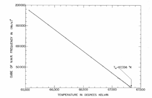
The results are known analytically, while the results are known only numerically (to about 5 or 6 significant figures; I truncated early in the table above). Both the and results are also in fairly good agreement with experiment, which confirm that the observed exponents do not take their mean field values. For example, the left-hand figure above shows the magnetisation taken from MnF, a magnet with uniaxial anisotropy which is thought to be described by the Ising model22 2 This data is taken from P. Heller and G. Benedek, Nuclear Magnetic Resonance in MnF Near the Critical Point, Phys. Rev. Lett. 8, 428 (1962).. The data shows a good fit to ; as shown in the table, it is now thought that the exponent is not a rational number, but .
This kind of behaviour is very surprising. It’s rare that we see any kind of non-analytic behaviour in physics, but rarer still to find exponents that are not integers or simple fractions. What is going on here? This is one of the questions we will answer as these lectures progress.
1.2.4 A First Look at Universality

Before we go digging further into the Ising model, there is one other important aspect that deserves a mention at this point. The phase diagram for the Ising model is rather similar to the phase diagram for the transition between a liquid and gas, now drawn in the pressure-temperature plane. This is shown in the figure. In both cases, there is a line of first order transitions, ending at a critical point. For water, the critical point lies at a temperature and a pressure atm.
The similarities are not just qualitative. One can use an appropriate equation of state for an interacting gas – say, the van der Waals equation – to compute how various quantities behave as we approach the critical point. (See the lectures on Statistical Physics for details of these calculations.) As we cross the first order phase transition, keeping the pressure constant, the volume of the liquid/gas jumps discontinuously. This suggests that the rescaled volume , where is the number of atoms in the gas, is analogous to in the Ising model. We can then ask how the jump in changes as we approach the critical point. One finds,
From the phase diagram, we see that the pressure is analogous to the magnetic field . We could then ask how the volume changes with pressure as we approach the critical point keeping fixed. We find
Finally, we want the analog of the magnetic susceptibility. For a gas, this is the compressibility, . As we approach the critical point, we find
It has probably not escaped your attention that these critical exponents are exactly the same as we saw for the Ising model when treated in mean field. The same is also true for the heat capacity which approach different constant values as the critical point is approached from opposite sides.
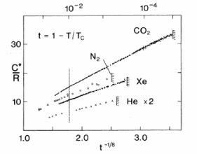
However, the coincidence doesn’t stop there. Because, it turns out, that the critical exponents above are also wrong! The true critical exponents for the liquid-gas transitions in and dimensions are the same as those of the Ising model, listed previously in the table. For example, experimental data for the critical exponent of a number of different gases was plotted two pages back33 3 The data is taken from J. Lipa, C. Edwards, and M. Buckingham Precision Measurement of the Specific Heat of CO Near the Critical Point”, Phys. Rev. Lett. 25, 1086 (1970). This was before the theory of critical phenomena was well understood. The data shows a good fit with , not too far from the now accepted value . Notice that the data stops around . This is apparently because the effect of gravity becomes important as the critical point is approached, making experiments increasingly difficult. showing that it is approximately , and certainly not consistent with mean field expectations.
This is an astonishing fact. It’s telling us that at a second order phase transition, all memory of the underlying microscopic physics is washed away. Instead, there is a single theory which describes the physics at the critical point of the liquid-gas transition, the Ising model, and many other systems. This is a theoretical physicist’s dream! We spend a great deal of time trying to throw away the messy details of a system to focus on the elegant essentials. But, at a critical point, Nature does this for us. Whatever drastic “spherical cow” approximation you make doesn’t matter: if you capture the correct physics, you will get the exact answer! The fact that many different systems are described by the same critical point is called universality.
We might ask: does every second order phase transition have the same critical exponents as the Ising model? The answer is no! Instead, in each dimension there is a set of critical points. Any system that undergoes a second order phase transition is governed by one member of this set. If two systems are governed by the same critical point, we say that they lie in the same universality class. The choice of universality class is, in large part, dictated by the symmetries of the problem; we will see some examples in Section 4.
The Ising Model as a Lattice Gas
It is, at first sight, surprising that a magnet and gas lie in the same universality class. However, there is a different interpretation of the Ising model that makes it look a little more gassy.
To see this, consider the same -dimensional lattice as before, but now with particles hopping between lattice sites. These particles have hard cores, so no more than one can sit on a single lattice site. We introduce the variable to specify whether a given lattice site, labelled by , is empty () or filled (. We can also introduce an attractive force between atoms by offering them an energetic reward if they sit on neighbouring sites. The Hamiltonian of such a lattice gas is given by
where is the chemical potential which determines the overall particle number. But this Hamiltonian is trivially the same as the Ising model (1.1) if we make the identification
The chemical potenial in the lattice gas plays the role of magnetic field in the spin system while the magnetization of the system (1.6) measures the average density of particles away from half-filling.
There’s no a priori reason to think that the Ising model is a particular good description of a gas. Nonetheless, this interpretation may make it a little less surprising that the Ising model and a gas share the same critical point.
1.3 Landau-Ginzburg Theory
The idea of universality – that many different systems enjoy the same critical point – is a powerful one. It means that if we want to accurately describe the critical point, we needn’t concern ourselves with the messy details of any specific system. Instead, we should just search for the simplest model which gives the correct physics and work with that.
What is the simplest model? The Landau approach – in which the configuration of the Ising model is reduced to a single number – is too coarse. This is because it misses any spatial variation in the system. And, as we will see shortly, the critical point is all about spatial variations. Here we describe a simple generalisation of Landau’s ideas which allows the system to move away from a homogeneous state. This generalisation is known as Landau-Ginzburg theory44 4 It is also known as Ginzburg-Landau theory. The original paper, dating from 1950, has the authors in alphabetical order and constructs the free energy of a superconductor. Here we use the term Landau-Ginzburg theory to reflect the fact that, following Landau’s earlier work, these ideas apply more broadly to any system..
The key idea is simple: we take the order parameter from Landau theory – which, for the Ising model, is the magnetisation – and promote it to a field which can vary in space, . This is referred to as a local order parameter.

How do we do this? We started with a lattice. We divide this lattice up many into boxes, with sides of length . Each of these boxes contains many lattice sites – call it – but the box size is smaller than any other length scale in the game. (In particular, should be smaller than something called the correlation length that we will encounter below.) For each box, we define the average magnetisation , where denotes the centre of the box. This kind of procedure in known as coarse-graining.
There are all sorts of subtleties involved in this construction, and we will do our best to sweep them firmly under the rug. First, takes values only at certain values of which label the positions of boxes. To mitigate this, we take the number of boxes to be big enough so that can be treated as a continuous variable. Second, at each , is quantised in units of . We will take big enough so that can take any value in . The upshot of this is that we will treat as a continuous function. However, we will at some point need to remember that it makes no sense for to vary on very short distance scales – shorter than the separation between boxes.
You may have noticed that we’ve not been particularly careful about defining and this cavalier attitude will continue below. You might, reasonably ask: does the physics depend on the details of how we coarse grain? The answer is no. This is the beauty of universality. We’ll see this more clearly as we proceed.
Our next step is to repeat the ideas that we saw in Section 1.1.1. Following (1.7), we write the partition function as
| (1.24) |
Here, the notation means that we sum over all configurations of spins such that the coarse graining yields . In general, there will be many spin configurations for each . We then sum over all possible values of .
This procedure has allowed us to define a free energy . This is a functional, meaning that you give it a function and it spits back a number, . This is known as the Landau-Ginzburg free energy
We will invoke one last notational flourish. We’re left in (1.24) with a sum over all possible configurations . With the assumption that is a continuous function, this is usually written as
| (1.25) |
This is a functional integral, also known as a path integral. The notation – which is usually shortened to simply – means that we should sum over all field configurations .
Path integrals may be somewhat daunting at first sight. But it’s worth remembering where it comes from: an integration over at each point labelling a box. In other words, it’s nothing more than an infinite number of normal integrals. We will start to learn how to play with these objects in Section 2.
The path integral looks very much like a usual partition function, but with the Landau-Ginzburg free energy playing the role of an effective Hamiltonian for the continuous variable . There is some nice intuition behind this. In the thermal ensemble, a given field configuration arises with probability
| (1.26) |
The path integral (1.25), is nothing but the usual partition function, now for a field rather than the more familiar variables of classical physics like position and momentum. In other words, we’re doing the statistical mechanics of fields, rather than particles. The clue was in the title of these lectures.
1.3.1 The Landau-Ginzburg Free Energy
The next step is to ask: how do we calculate ? This seems tricky: already in our earlier discussion of Landau theory, we had to resort to an unjustified mean field approximation. What are we going to do here?
The answer to this question is wonderfully simple, as becomes clear if we express the question in a slightly different way: what could the free energy possibly be? There are a number of constraints on that arise from its microscopic origin
-
•
Locality: The nearest neighbour interactions of the Ising model mean that a spin on one site does not directly affect a spin on a far flung site. It only does so through the intermediate spins. The same should be true of the magnetisation field . The result is that the free energy should take the form
where is a local function. It can depend on , but also on and higher derivatives. These gradient terms control how the field at one point affects the field at neighbouring points.
-
•
Translation and Rotation Invariance: The original lattice has a discrete translation symmetry. For certain lattices (e.g. a square lattice) there can be discrete rotation symmetries. At distances much larger than the lattice scale, we expect that the continuum version of both these symmetries emerges, and our free energy should be invariant under them.
-
•
symmetry. When , the original Ising model (1.1) is invariant under the symmetry , acting simultaneously on all sites. This symmetry is inherited in our coarse-grained description which should be invariant under
(1.27) When , the Ising model is invariant under , together with . Again, our free energy should inherit this symmetry.
-
•
Analyticity: We will make one last assumption: that the free energy density is an analytic function of and its derivatives. Our primary interest lies in the critical point where first becomes non-zero, although we will also use this formalism to describe first order phase transitions where is small. In both cases, we can Taylor expand the free energy in and restrict attention to low powers of .
Furthermore, we will restrict attention to situations where varies rather slowly in space. In particular, we will assume that varies appreciably only over distances that are much larger than the distance between boxes. This means that we can also consider a gradient expansion of , in the dimensionless combination . This means that terms are more important than terms and so on.
With these considerations in place, we can now simply write down the general form of the free energy. When , the symmetry (1.27) means that the free energy can depend only on even powers of . The first few terms in the expansion are
| (1.28) |
There can also be a piece – like the that appeared in the Landau free energy – which doesn’t depend on the order parameter and so, for the most part, will play no role in the story. Notice that we start with terms quadratic in the gradient: a term linear in the gradient would violate the rotational symmetry of the system.
When , we can can have further terms in the free energy that are odd in , but also odd in , such as and . Each of these comes with a coefficient which is, in general, a function of .
The arguments that led us to (1.28) are very general and powerful; we will see many similar arguments in Section 4. The downside is that we are left with a bunch of unknown coefficients , and . These are typically hard to compute from first principles. One way forward is to import our results from Landau mean field approach. Indeed, for constant , the free energy (1.28) coincides with our earlier result (1.13) in Landau theory, with
| (1.29) |
Happily, however, the exact form of these functions will not be important. All we will need is that these functions are analytic in , and that and , while flips sign at the second order phase transition.
Looking ahead, there is both good news and bad. The good news is that the path integral (1.25), with Landau-Ginzburg free energy (1.28), does give a correct description of the critical point, with the surprising -dependent critical exponents described in Section 1.2.3. The bad news is that this path integral is hard to do! Here “hard” means that many of the unsolved problems in theoretical physics can be phrased in terms of these kinds of path integrals. Do not fear. We will tread lightly.
1.3.2 The Saddle Point and Domain Walls
We are going to build up slowly to understand how we can perform the functional integral (1.25). As a first guess, we’ll resort to the saddle point method and assume that the path integral is dominated by the configurations which minimise . In subsequent sections, we’ll treat the integral more seriously and do a better job.
To find the minima of functionals like , we use the same kind of variational methods that we met when working with Lagrangians in Classical Dynamics . We take some fixed configuration and consider a nearby configuration . The change in the free energy is then
where, to go from the first line to the second, we have integrated by parts. This encourages us to introduce the functional derivative,
Note that I’ve put back the dependence to stress that, in contrast to , is evaluated at some specific position .
If the original field configuration was a minimum of the free energy it satisfies the Euler-Lagrange equations,
| (1.30) |
The simplest solutions to this equation have constant. This recovers our earlier results from Landau theory. When , we have and the ground state has . In contrast, when , and there is a degenerate ground state with
| (1.31) |
This is the same as our previous expression (1.14), where we replaced and with the specific functions (1.29). We see that what we previously called the mean field approximation, is simply the saddle point approximation in Landau-Ginzburg theory. For this reason, the term “mean field theory” is given to any situation where we write down the free energy, typically focussing on a Taylor expansion around , and then work with the resulting Euler-Lagrange equations.
Domain Walls
The Landau-Ginzburg theory contains more information than our earlier Landau approach. It also tells us how the magnetisation changes in space.
Suppose that we have so there exist two degenerate ground states, . We could cook up a situation in which one half of space, say , lives in the ground state while the other half of space, lives in . The two regions in which the spins point up or down are called domains. The place where these regions meet is called the domain wall.
We would like to understand the structure of the domain wall. How does the system interpolate between these two states? The transition can’t happen instantaneously because that would result in the gradient term giving an infinite contribution to the free energy. But neither can the transition linger too much because any point at which differs significantly from the value costs free energy from the and terms. There must be a happy medium between these two.
To describe the system with two domains, must vary but it need only change in one direction: . Equation (1.30) then becomes an ordinary differential equation,
This equation is easily solved. If we insist that the field interpolate between the two different ground states, as , then the solution is given by
| (1.32) |

This is plotted in the figure. Here is the position of the domain wall and
is its width. For , the magnetisation relaxes exponentially quickly back to the ground state values .
We can also compute the cost in free energy due to the presence of the domain wall. To do this, we substitute the solution back into the expression for the free energy (1.28). The cost is not proportional to the volume of the system, but instead proportional to the area of the domain wall. This means that if the system has linear size then the free energy of the ground state scales as while the additional free energy required by the wall scales only as . It is simple to see that the excess cost in free energy of the domain wall has parametric dependence
| (1.33) |
Here’s the quick way to see this: from the solution (1.32), the field changes by over a distance . This means that and the gradient term in the free energy contributes , where the second expression comes because the support of the integral is only non-zero over the width where the domain wall is changing. This gives the parametric dependence (1.33). There are further contributions from the and terms in the potential, but our domain wall solves the equation of motion whose purpose is to balance the gradient and potential terms. This means that the potential terms contribute with the same parametric dependence as the gradient terms, a fact you can check by hand by plugging in the solution.
Notice that as we approach the critical point, and , the two vacua are closer, the width of the domain wall increases and its energy decreases.
1.3.3 The Lower Critical Dimension
We stated above that the Ising model has no phase transition in dimensions. The reason behind this can be traced to the existence of domain walls, which destroy any attempt to sit in the ordered phase.
Let’s set where we would expect two, ordered ground states . To set up the problem, we start by considering the system on a finite interval of length . At one end of this interval – say the left-hand edge – we’ll fix the magnetisation to be in its ground state . One might think that the preferred state of the system is then to remain in everywhere. But what actually happens?
There is always a probability that a domain wall will appear in the thermal ensemble and push us over to the other ground state . The probability for a wall to appear at some point is given by (1.26)
This looks like it’s exponentially suppressed compared to the probability of staying put. However, we get an enhancement because the domain wall can sit anywhere on the line . This means that the probability becomes
For a large enough system, the factor of will overwhelm any exponential suppression. This is an example of the entropy of a configuration – which, in this context is – outweighing the energetic cost.
Of course, once we’ve got one domain wall there’s nothing to stop us having another, flipping us back to . If we have an even number of domain walls along the line, we will be back at by the time we get to the right-hand edge at ; an odd number and we’ll sit in the other vacuum . Which of these is most likely?
The probability to have walls, placed anywhere, is
This means that the probability that we start at and end up at is
Meanwhile, the probability that the spin flips is
We see that, at finite , there is some residual memory of the boundary condition that we imposed on the left-hand edge. However, as , this gets washed away. You’re just as likely to find the spins up as down on the right-hand edge.
Although we phrased this calculation in terms of pinning a choice of ground state on a boundary, the same basic physics holds on an infinite line. Indeed, this is a general principle: whenever we have a Landau-Ginzburg theory characterised by a discrete symmetry – like the of the Ising model – then the ordered phase will have a number of degenerate, disconnected ground states which spontaneously break the symmetry. In all such cases, the lower critical dimension is and in all cases the underlying reason is the same: fluctuations of domain walls will take us from one ground state to another and destroy the ordered phase. It is said that the domain walls proliferate.
We could try to run the arguments above in dimensions . The first obvious place that it fails is that the free energy cost of the domain wall (1.33) now scales with the system size, . This means that as increases, we pay an exponentially large cost from . Nonetheless, one could envisage a curved domain wall, which encloses some finite region of the other phase. It turns out that this is not sufficient to disorder the system. However, in , the fluctuations of the domain wall become important as one approaches the critical point.
1.3.4 Lev Landau: 1908-1968
Lev Landau was one of the great physicists of the 20th century. He made important contributions to nearly all areas of physics, including the theory of magnetism, phase transitions, superfluids and superconductors, Fermi liquids and quantum field theory. He founded a school of Soviet physics whose impact lasts to this day.
Landau was, by all accounts, boorish and did not suffer fools gladly. This did not sit well with the authorities and, in 1938, he was arrested in one of the great Soviet purges and sentenced to 10 years in prison. He was rescued by Kapitza who wrote a personal letter to Stalin arguing, correctly as it turned out, that Landau should be released as he was the only person who could understand superfluid helium. Thus, for his work on superfluids, Landau was awarded both his freedom and, later, the Nobel prize. His friend, the physicist Yuri Rumer, was not so lucky, spending 10 years in prison before exile to Siberia.

Legend has it that Landau hated to write. The extraordinarily ambitious, multi-volume “Course on Theoretical Physics” was entirely written by his co-author Evgeny Lifshitz, usually dictated by Landau. As Landau himself put it: ”Evgeny is a great writer: he cannot write what he does not understand”.
Here is a story about a visit by Niels Bohr to Landau’s Moscow Institute. Bohr was asked by a journalist how he succeeded in creating such a vibrant atmosphere in Copenhagen. He replied “I guess the thing is, I’ve never been embarrassed to admit to my students that I’m a fool”. This was translated by Lifshitz as: “I guess the thing is, I’ve never been embarrassed to admit to my students that they’re fools”. According to Kapista, the translation was no mistake: it simply reflected the difference between Landau’s school and Bohr’s.
In 1962, Landau suffered a car accident. He survived but never did physics again.