3 The Renormalisation Group

We’ve built up the technology of field theory and path integrals, and I’ve promised you that this is sufficient to understand what happens at a second order phase transition. But so far, we’ve made little headway. All we’ve seen is that as we approach the critical point, fluctuations dominate and the Gaussian path integral is no longer a good starting point. We need to take the interactions into account.

Sometimes in physics, you can understand a phenomenon just by jumping in and doing the right calculation. And we will shortly do this, using perturbation theory to understand how the $\phi^{4}$ terms change the critical exponents. However, to really understand second order phase transitions requires something more: we will need to set up the right framework in which to think of physics at various length scales. This set of ideas was developed in the 1960s and 1970s, by people like Leo Kadanoff, Michael Fisher and, most importantly, Kenneth Wilson. It goes by the name of the Renormalisation Group.

3.1 What’s the Big Idea?

Let’s start by painting the big picture. As in the previous section, we’re going to consider a class of theories based around a single scalar field $\phi({{\bf x}})$ in $d$ dimensions. (We will consider more general set-ups in Section 4.) The free energy takes the now familiar form,

\displaystyle F[\phi]=\int d^{d}x\ \left[\frac{1}{2}\nabla\phi\cdot\nabla\phi+% \frac{1}{2}\mu^{2}\phi^{2}+g\phi^{4}+\ldots\right]

(3.65)

In what follows, we will look at what happens as we approach the critical point from above $T\rightarrow T_{c}$ . All the important temperature dependence in (3.65) is sitting in the quadratic term, with

\displaystyle\mu^{2}\sim T-T_{c}

(3.66)

In contrast to the previous section, we will allow $\mu^{2}$ to take either sign: $\mu^{2}>0$ in the disordered phase, and $\mu^{2}<0$ in the ordered phase where $\langle\phi\rangle\neq 0$ .

There is one important change in convention from our earlier discussion: we have rescaled the coefficient of the gradient term to be $1/2$ ; we will see the relevance of this shortly. All other terms have arbitrary coefficients.

So far we’ve focussed on just a few couplings, as shown in the free energy (3.65). Here we’re going to expand our horizons. We’ll consider all possible terms in the free energy, subject to a couple of restrictions. We’ll insist that the free energy is analytic around $\phi=0$ , so has a nice Taylor expansion, and we will insist on the ${\bf Z}_{2}$ symmetry $\phi\rightarrow-\phi$ , so that only even powers of $\phi$ arise. This means, for example, that we will include the term $\phi^{6}$ and $(\nabla^{2}\phi)^{2}$ and $\phi^{14}$ and $\phi^{137}(\nabla\phi\cdot\nabla\phi)\nabla^{2}\phi$ and so so. Each of these terms comes with its own coupling constant. However, we don’t include terms like $\phi^{17}$ because this violates the ${\bf Z}_{2}$ symmetry, nor $1/\phi^{2}$ because this is not analytic at $\phi=0$ .

Next, consider the infinite dimensional space, parameterised by the infinite number of coupling constants. We will call this the theory space (although I should warn you that this isn’t standard terminology). You should have in your mind something like this:

But possibly bigger.

As we’ve seen, our interest is in computing the partition function

\displaystyle Z=\int{\cal D}\phi\ e^{-F[\phi]}

(3.67)

Note that I’ve written the exponent as $e^{-F}$ rather than $e^{-\beta F}$ . This is because the overall power of $\beta$ does nothing to affect the physics; all the relevant temperature dependence is in the coefficient (3.66) while, for the quantities of interest near the critical point, this overall factor can be set to $\beta\approx 1/T_{c}$ . You can think that we’ve simply rescaled this into the field $\phi$ .

There is one more ingredient that we need to make sense of the path integral (3.67). This is the UV cut-off $\Lambda$ . Recall that, implicit in our construction of the theory is the requirement that the Fourier modes $\phi_{\bf k}$ vanish for suitably high momenta

\displaystyle\phi_{\bf k}=0\ \ \ {\rm for}\ k>\Lambda

This arises because, ultimately our spins sit on some underlying lattice which, in turn, was coarse-grained into boxes of size $a$ . The UV cut-off is given by $\Lambda\sim 1/a$ .

Until now, the UV cut-off has taken something of a back seat in our story, although it was needed to render some of the path integral calculation in the previous section finite. Now it’s time for $\Lambda$ to move centre stage. As we will explain, we can use the cut-off to define a flow in the space of theories.

Suppose that we only care about physics on long distance scales, $L$ . Then we have no real interest in the Fourier modes $\phi_{\bf k}$ with $k\gg 1/L$ . This suggests that we can write down a different theory, that has a lower cut-off,

\displaystyle\Lambda^{\prime}=\frac{\Lambda}{\zeta}

for some $\zeta$ . As long as $\Lambda^{\prime}\gg 1/L$ , the scale of interest, our theory can tell us everything that we need to know. Moreover, we know, at least in principle, how to construct such a theory. We write our Fourier modes as

\displaystyle\phi_{\bf k}=\phi^{-}_{\bf k}+\phi^{+}_{\bf k}

where $\phi_{\bf k}^{-}$ describe the long-wavelength fluctuations

\displaystyle\phi_{\bf k}^{-}=\left\{\begin{array}[]{cc}\phi_{\bf k}&k<\Lambda% ^{\prime}\\ 0&k>\Lambda^{\prime}\end{array}\right.

and $\phi_{\bf k}^{+}$ describe the short-wavelength fluctuations that we don’t care about

\displaystyle\phi_{\bf k}^{+}=\left\{\begin{array}[]{cc}\phi_{\bf k}&\Lambda^{% \prime}<k<\Lambda\\ 0&\mbox{otherwise}\end{array}\right.

There are several other names for these variables that are used interchangeably. The modes $\phi_{\bf k}^{-}$ and $\phi_{\bf k}^{+}$ are also referred to as low- and high-energy modes or, importing language from quantum mechanics, slow and fast modes, respectively. In a rather quaint nod to the electromagnetic spectrum, the short-distance, microscopic physics that we care little about is often called the ultra-violet; the long-distance physics that we would like to understand is the infra-red.

Similarly, we decompose the free energy, written in Fourier space, as

\displaystyle F[\phi_{{\bf k}}]=F_{0}[\phi_{{\bf k}}^{-}]+F_{0}[\phi_{{\bf k}}% ^{+}]+F_{I}[\phi_{{\bf k}}^{-},\phi_{{\bf k}}^{+}]

Here $F_{I}[\phi_{{\bf k}}^{-},\phi_{{\bf k}}^{+}]$ involves the terms which mix the short and long-wavelength modes. The partition function (3.67) can then be written as

\displaystyle Z=\int\prod_{k<\Lambda}d\phi_{{\bf k}}\ e^{-F}=\int\prod_{k<% \Lambda^{\prime}}d\phi_{{\bf k}}^{-}\ e^{-F_{0}[\phi_{{\bf k}}^{-}]}\int\prod_% {\Lambda^{\prime}<k<\Lambda}d\phi_{{\bf k}}^{+}\ e^{-F_{0}[\phi_{{\bf k}}^{+}]% }e^{-F_{I}[\phi_{{\bf k}}^{-},\phi_{{\bf k}}^{+}]}

We write this as

\displaystyle Z=\int{\cal D}\phi^{-}\ e^{-F^{\prime}[\phi^{-}]}

where $F^{\prime}[\phi]$ is known as the Wilsonian effective free energy. (In fairness, this term is rarely used: you’re more likely to hear “Wilsonian effective action” to describe the analogous object in a path integral describing a quantum field theory.) We’re left with a free energy which describes the long-wavelength modes, but takes into account the effects of the short wavelength modes. It is defined by

\displaystyle e^{-F^{\prime}[\phi^{-}]}=e^{-F_{0}[\phi_{{\bf k}}^{-}]}\int% \prod_{\Lambda^{\prime}<k<\Lambda}d\phi_{{\bf k}}^{+}\ e^{-F_{0}[\phi_{{\bf k}% }^{+}]}e^{-F_{I}[\phi_{{\bf k}}^{-},\phi_{{\bf k}}^{+}]}

(3.68)

In subsequent sections, we’ll put some effort into calculating this object. However, at the end of the day the new free energy $F^{\prime}[\phi^{-}]$ must take the same functional form as the original free energy (3.65), simply because we started from the most general form possible. The only effect of integrating out the high-momentum modes is to shift the infinite number of coupling constants, so we now have

\displaystyle F^{\prime}[\phi]=\int d^{d}x\ \left[\frac{1}{2}\gamma^{\prime}% \nabla\phi\cdot\nabla\phi+\frac{1}{2}\mu^{\prime\,2}\phi^{2}+g^{\prime}\phi^{4% }+\ldots\right]

(3.69)

We would like to compare the new free energy (3.69) with the original (3.65). However, we’re not quite there yet because, the two theories are different types of objects – like apples and oranges – and shouldn’t be directly compared. This is because the theory is defined by both the free energy and the UV cut-off and, by construction our two theories have different cut-offs. This means that the original theory $F[\phi]$ can describe things that the new theory $F^{\prime}[\phi^{-}]$ cannot, namely momentum modes above the cut-off $\Lambda^{\prime}$ .

It is straightforward to remedy this. We can place the two theories on a level playing field by rescaling the momenta in the new theory. We define

\displaystyle{\bf k}^{\prime}=\zeta{\bf k}

Now $k^{\prime}$ takes values up to $\Lambda$ , as did $k$ in the original theory. The counterpart of this scaling in real space is

\displaystyle{\bf x}^{\prime}=\frac{{\bf x}}{\zeta}

This means that all lengths scales are getting smaller. You can think of this step as zooming out, to observe the system on larger and larger length scales. As you do so, all features become smaller.

There is one final step that we should take. The new theory $F^{\prime}[\phi]$ will typically have some coefficient $\gamma^{\prime}\neq 1$ in front of the leading, quadratic gradient term. To compare with the original free energy (3.65), we should rescale our field. We define

\displaystyle\phi^{\prime}_{{\bf k}^{\prime}}={\sqrt{\gamma^{\prime}}}\,\phi^{% -}_{{\bf k}}

Which, in position space, reads

\displaystyle\phi^{\prime}({\bf x}^{\prime})=\sqrt{\gamma^{\prime}}\,\phi^{-}(% {\bf x})

(3.70)

Now, finally, our free energy takes the form

\displaystyle F_{\zeta}[\phi^{\prime}]=\int d^{d}x\ \left[\frac{1}{2}\nabla% \phi^{\prime}\cdot\nabla\phi^{\prime}+\frac{1}{2}\mu^{2}(\zeta)\phi^{\prime\,2% }+g(\zeta)\phi^{\prime\,4}+\ldots\right]

(3.71)

We see that this procedure induces a continuous map from $\zeta\in[1,\infty)$ onto the space of coupling constants. Our original coupling constants in (3.65) are those evaluated at $\zeta=1$ . As we increase $\zeta$ , we trace out curves in our theory space, that look something like the picture shown in Figure 22

We say that the coupling constants flow, where the direction of the flow is telling us what the couplings look like on longer and longer length scales. The equations which describe these flows – which we will derive shortly – are known, for historic reasons, as beta functions.

Figure 22: Flows in theory space; the arrows are in the direction of increasing

\zeta

These, then are the three steps of what is known as the renormalisation group (RG):

•

Integrate out high momentum modes, $\Lambda/\zeta<k<\Lambda$ .
•

Rescale the momenta ${\bf k}^{\prime}=\zeta{\bf k}$ .
•

Rescale the fields so that the gradient term remains canonically normalised.

You may wonder why we didn’t just include a coupling constant $\gamma(\zeta)$ for the gradient term, and watch that change too. The reason is that we can always scale this away by redefining $\phi$ . But $\phi$ is just a dummy variable which is integrated over the path integral, so this rescaling can’t change the physics. To remove this ambiguity, we should pin down the value of one of the coupling constants, and the gradient term $(\nabla\phi)^{2}$ is the most convenient choice. If we ever find ourselves in a situation where $\gamma(\zeta)=0$ for some $\zeta$ then we would have to re-evaluate this choice. (We’ll actually come across an example where it’s sensible to make a different choice in Section 4.3.)

The “renormalisation group” is not a great name. It has a hint of a group structure, because a scaling by $\zeta_{1}$ followed by a scaling by $\zeta_{2}$ gives the same result as a scaling by $\zeta_{1}\zeta_{2}$ . However, unlike for groups, there is no inverse: we can only integrate out fields, we can’t put them back in. A more accurate name would be the “renormalisation semi-group”.

The Renormalisation Group in Real Space

The procedure we’ve described above is the renormalisation group in momentum space: to get an increasingly coarse-grained description of the physics, we integrate out successive momentum shells. This version of the renormalisation group is most useful when dealing with continuous fields and will be the approach we will focus on in this course.

There is a somewhat different, although ultimately equivalent, phrasing of the renormalisation group which works directly in real space. This approach works best when dealing directly with lattice systems, like the Ising model. As we explained rather briefly in Section 1.3, one constructs a magnetisation field $m({{\bf x}})$ by coarse-graining over boxes of size $a$ , each of which contains many lattice sites. One can ask how the free energy changes as we increase $a$ , a procedure known as blocking. Ultimately this leads to the same picture that we built above.

3.1.1 Universality Explained

Even before we do any calculations, there are general lessons to be extracted from the framework above. Let’s suppose we start from some point in theory space. This can be arbitrarily complicated, reflecting the fact that it contains informations about all the microscopic, short-distance degrees of freedom.

Of course, we care little about most of these details so, in an attempt to simplify our lives we perform a renormalisation group transformation, integrating out short distance degrees of freedom to generate a new theory which describes the long wavelength physics. And then we do this again. And then we do this again. Where do we end up?

There are essentially two possibilities: we could flow off to infinity in theory space, or we could converge towards a fixed point. These are points which are invariant under a renormalisation group transformation. (One could also envisage further possibilities, such as converging towards a limit cycle. It turns out that these can be ruled out in many theories of interest.)

Our interest here lies in the fixed points. The second step in the renormalisation group procedure ensures that fixed points describe theories that have no characteristic scale. If the original theory had a correlation length scale $\xi$ , then the renormalised theory has a length scale $\xi^{\prime}=\xi/\zeta$ . (We will derive this statement explicitly below when we stop talking and start calculating.) Fixed points must therefore have either $\xi=0$ or $\xi=\infty$ .

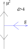
In the disordered phase, with $T>T_{c}$ , enacting an RG flow reduces the correlation length. Pictorially, we have

\displaystyle\raisebox{-32.25pt}{\epsfbox{sftfigs/isingdis.eps}}\ \ \ \ % \xrightarrow{\mbox{RG flow}}\ \ \ \ \raisebox{-32.25pt}{\epsfbox{sftfigs/ising% 600.eps}}

In this case, shrinking the correlation length is equivalent to increasing the temperature. The end point of the RG flow, at $\xi=0$ , is the infinite temperature limit of the theory. This is rather like flowing off to infinity in theory space. As we will see, it is not uncommon to end up here after an RG flow. But it is boring.

Similarly, in the ordered phase the RG flow again reduces the correlation length,

\displaystyle\raisebox{-32.25pt}{\epsfbox{sftfigs/isinglow.eps}}\ \ \ \ % \xrightarrow{\mbox{RG flow}}\ \ \ \ \raisebox{-32.25pt}{\epsfbox{sftfigs/% isinglower.eps}}

Now the end point at $\xi=0$ corresponds to the zero temperature limit; again, it is a typical end point of RG flow but is dull.

Theories with $\xi=\infty$ are more interesting. As we saw above, this situation occurs at a critical point where the theory contains fluctuations on all length scales. Now, if we do an RG flow, the theory remains invariant. In terms of our visual configurations,

\displaystyle\raisebox{-32.25pt}{\epsfbox{sftfigs/ising227.eps}}\ \ \ \ % \xrightarrow{\mbox{RG flow}}\ \ \ \ \raisebox{-32.25pt}{\epsfbox{sftfigs/% isingcrit2.eps}}

Note that the configuration itself doesn’t stay the same. (It is, after all, merely a representative configuration in the ensemble.) However, as the fluctuations on small distance scales shrink away due to RG, they are replaced by fluctuations coming in from larger distance scales. The result is a theory which is scale invariant. For this reason, the term “critical point” is often used as a synonym for “fixed point” of the RG flow.

Figure 23: The critical surface. Irrelevant deformations from the critical point are shown as dotted blue lines; the relevant deformation is is red.

This picture is all we need to understand the remarkable phenomenon of universality: it arises because many points in theory space flow to the same fixed point. Thus, many different microscopic theories have the same long distance behaviour.

Relevant, Irrelevant or Marginal

It is useful to characterise the properties of fixed points by thinking about the theories in their immediate neighbourhood. Obviously, there are an infinite number of ways we can move away from the fixed point. If we move in some of these directions, the RG flow will take us back towards the fixed point. These deformations are called irrelevant because if we add any such terms to the free energy we will end up describing the same long-distance physics.

In contrast, there will be some directions in which the RG flow will sweep us away from the fixed point. These deformations are called relevant because if we add any such terms to the free energy, the long-distance physics will be something rather different. Examples of relevant and irrelevant deformations are shown in Figure 23. Much of the power of universality comes from the realisation that the vast majority of directions are irrelevant. For a given fixed point, there are typically only a handful of relevant deformations, and an infinite number of irrelevant ones. This means that our fixed points have a large basin of attraction, huge slices of the infinite dimensional theory space all converging to the same fixed point. The basin of attraction for a particular fixed point is called the critical surface.

Finally, it’s possible that our fixed point is not a point at all, but a line or a higher dimensional surface living within theory space. In this case, if we deform the theory in the direction of the line, we will not flow anywhere, but simply end up on another fixed point. Such deformations are called marginal; they are rare, but not unheard of.

Why High Energy Physics is Hard

Universality is a wonderful thing if you want to understand the low-energy, long-wavelength physics. It tells you that you can throw away many of the microscopic details because they are irrelevant for the things that you care about.

In contrast, if you want to understand the high-energy, short distance physics then universality is the devil. It tells you that you have very little hope of extracting any information about microscopic degrees of freedom if you only have access to information at long distances. This is because many different microscopic theories will all give the same answer.

As we saw in Section 2.3, quantum field theory is governed by the same mathematical structure as statistical field theory, and the comments above also apply. Suppose, for example, that you find yourself living in a technologically adolescent civilisation that can perform experiments at distance scales of $10^{-16}$ cm or so, but no smaller. Yet, what you really care about is physics at, say, $10^{-32}$ cm where you suspect that something interesting is going on. The renormalisation group says that you shouldn’t pin your hopes on learning anything from experiment.

The renormalisation group isn’t alone in hiding high-energy physics from us. In gravity, cosmic censorship ensures that any high curvature regions are hidden behind horizons of black holes while, in the early universe, inflation washes away any trace of what took place before. Anyone would think there’s some kind of conspiracy going on….

3.2 Scaling

The idea that second order phase transitions coincide with fixed points of the renormalisation group is a powerful one. In particular, it provides an organising principle behind the flurry of critical exponents that we met in Section 1.

As we explained above, at a fixed point of the renormalisation group any scale must be washed away. This is already enough to ensure that correlation functions must take the form of a power-law,

\displaystyle\langle\phi({{\bf x}})\phi(0)\rangle\sim\frac{1}{r^{d-2+\eta}}

(3.72)

Any other function would require a scale on dimensional grounds. The only freedom that we have is in the choice of exponent which we have chosen to parameterise as $\eta$ . One of the tasks of the RG procedure is to compute $\eta$ , and we will see how this works in Section 3.5.

However, even here there’s something of a mystery because usually we can figure out the way things scale by doing some simple dimensional analysis. (If you would like to refresh your memory, some examples of dimensional analysis can be found in Chapter 3 of the lectures on Dynamics and Relativity.) What does that tell us in the present case?

We will measure dimension in units of inverse length. So, for example, $[x]=-1$ while $[\partial/\partial x]=+1$ . The quantity $F[\phi]$ must be dimensionless because it sits in the exponent of the partition function as $e^{-F}$ . The first term is

\displaystyle F[\phi]=\int d^{d}x\ \frac{1}{2}\nabla\phi\cdot\nabla\phi+\ldots

From this we learn that

\displaystyle[\phi]=\frac{d-2}{2}

(3.73)

Which, in turn, tells us exactly what the exponent of the correlation function must be: $\eta=0$ .

This is sobering. Dimensional analysis is one of the most basic tools that we have, and yet it seems to be failing at critical points where experiment is showing that $\eta\neq 0$ . What’s going on?

A better way to think about dimensional analysis is to think in terms of scaling. Suppose that we rescale all length as ${\bf x}\rightarrow{\bf x}^{\prime}={\bf x}/\zeta$ . How should other quantities scale so that formula remains invariant? Stated this way, it’s clear that there’s a close connection between dimensional analysis and RG. The correlation function (3.72) is telling us that we should rescale $\phi({{\bf x}})\rightarrow\phi^{\prime}({\bf x}^{\prime})=\zeta^{\Delta_{\phi}% }\phi({{\bf x}})$ , where

\displaystyle\Delta_{\phi}=\frac{d-2+\eta}{2}

(3.74)

This is called the scaling dimension. It differs from the naive “engineering dimension” $[\phi]$ by the extra term $\eta/2$ which is referred to as the anomalous dimension.

We still haven’t explained why the scaling dimension differs from engineering dimension. The culprit turns out to be the third step of the RG procedure (3.70) where the field $\phi$ gets rescaled. In real space, this is viewed as coarse-graining $\phi$ over blocks of larger and larger size $a$ . As we do so, it dresses $\phi$ with this UV cut-off scale $\Lambda\sim 1/a$ , often in a complicated and non-intuitive way. This means that the correlation function (3.72) is actually

\displaystyle\langle\phi({{\bf x}})\phi(0)\rangle\sim\frac{a^{\eta}}{r^{d-2+% \eta}}

which is in full agreement with naive dimensional analysis. We can work with usual engineering dimensions if we keep track of this microscopic distance scale $a$ . But it is much more useful to absorb this into $\phi$ and think of a coarse-grained observable, with dimension $\Delta_{\phi}$ , that is the appropriate for measuring long distance correlations.

3.2.1 Critical Exponents Revisited

The critical exponents that we met in Section 1.2.3 are all a consequence of scale invariance, and dimensional analysis based on the scaling dimension. Let’s see how this arises.

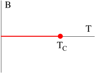
We know that as we move away from the critical point by turning on $\mu^{2}\sim T-T_{c}$ , we introduce a new length scale into the problem. This is the correlation length, given by

\displaystyle\xi\sim t^{-\nu}\ \ \ {\rm with}\ \ \ t=\frac{|T-T_{c}|}{T_{c}}

(3.75)

Here $t$ is called the reduced temperature, while $\nu$ is another critical exponent that we will ultimately have to calculate. Since $\xi$ is a length scale, it transforms simply as $\xi\rightarrow\xi/\zeta$ . In other words, it has scaling dimension $\Delta_{\xi}=-1$ . The meaning of the critical exponent $\nu$ is that the reduced temperature scales as $t\rightarrow\zeta^{\Delta_{t}}t$ , with

\displaystyle\Delta_{t}=\frac{1}{\nu}

(3.76)

In what follows, our only assumption is that the correlation length $\xi$ is the only length scale that plays any role.

We start with the thermodynamic free energy, $F_{\rm thermo}(t)$ , evaluated at $B=0$ . This takes the form

\displaystyle F_{\rm thermo}(t)=\int d^{d}x\ f(t)

Because $F_{\rm thermo}$ is scale invariant at the fixed point, $f(t)$ must have scaling dimension $d$ , which immediately tells us that

\displaystyle f(t)\sim t^{d\nu}

There is an intuitive way to understand this. At $T$ close to $T_{c}$ , the spins are correlated over distances scales $\xi$ , and can be viewed as moving as one coherent block. The free energy $F_{\rm thermo}$ is extensive, and so naturally scales as $F\sim(L/\xi)^{d}\sim t^{d\nu}$ .

From the thermodynamic free energy, we can compute the singular contribution to the heat capacity near $t=0$ . It is

\displaystyle c\sim\frac{\partial^{2}f}{\partial t^{2}}\sim t^{d\nu-2}\sim t^{% -\alpha}

where the second relationship is there to remind us that we already had a name for the critical exponent related to heat capacity. We learn that

\displaystyle\alpha=2-d\nu

(3.77)

This is called the Josephson relation or, alternatively, the hyperscaling relation.

The next critical exponent on the list is $\beta$ . Recall that this relates the magnetisation in the ordered phase – which we used to call $m$ and have now called $\phi$ – to the temperature as

\displaystyle\phi\sim t^{\beta}

But the scaling dimensions of this equation only work if we have

\displaystyle\Delta_{\phi}=\beta\Delta_{t}\ \ \ \Rightarrow\ \ \ \beta=\nu% \Delta_{\phi}=\frac{(d-2+\eta)\nu}{2}

(3.78)

The next two critical exponents require us to move away from the critical point by turning on a magnetic field $B$ . This is achieved through the addition of a linear term $\int d^{d}x\ B\phi$ in the free energy. (We didn’t include such a linear term in our previous discussion of RG, but it can be added without changing the essence of the story.) The scaling dimensions of this term must add to zero, giving

\displaystyle\Delta_{\phi}+\Delta_{B}=d\ \ \ \Rightarrow\ \ \ \ \Delta_{B}=% \frac{d+2-\eta}{2}

Now we can look at the various relationships. The behaviour of the susceptibility near the critical point is

\displaystyle\chi=\left.\frac{\partial{\phi}}{\partial{B}}\right|_{T}\sim t^{-\gamma}

Once again, the scaling dimensions are enough to fix $\gamma$ to be

\displaystyle\Delta_{\phi}-\Delta_{B}=-\frac{\gamma}{\nu}\ \ \ \Rightarrow\ \ % \ \gamma=\nu(2-\eta)

(3.79)

which is sometimes called Fisher’s identity. Once again, there is an intuitive way to understand this. The meaning of $\xi$ is that the spins are no longer correlated at distances $r\gg\xi$ . This can be seen, for example, in our original formula (2.62). Using our earlier expression (2.61) for the susceptibility, we have

\displaystyle\chi\sim\int_{0}^{\xi}d^{d}x\ \frac{1}{r^{d-2+\eta}}\sim\xi^{2-% \eta}\sim t^{-\nu(2-\eta)}

which again gives $\gamma=\nu(2-\eta)$ .

The final critical exponent relates the magnetisation $\phi$ to the magnetic field $B$ when we sit at the critical temperature $t=0$ . It should come as little surprise by now to learn that this is again fixed by scaling analysis

\displaystyle\phi\sim B^{1/\delta}\ \ \ \Rightarrow\ \ \ \delta=\frac{\Delta_{% B}}{\Delta_{\phi}}=\frac{d+2-\eta}{d-2+\eta}

(3.80)

We end up with four equations, relating $\alpha$ (3.77), $\beta$ (3.78), $\gamma$ (3.79) and $\delta$ (3.80) to the critical exponents $\eta$ and $\nu$ . For convenience, let’s recall what values we claimed this exponents take:

	$\alpha$	$\beta$	$\gamma$	$\delta$	$\eta$	$\nu$
MF	$\frac{4-d}{2}$	$\frac{1}{2}$	1	3	0	$\frac{1}{2}$
$d=2$	0	$\frac{1}{8}$	$\frac{7}{4}$	15	$\frac{1}{4}$	1
$d=3$	0.1101	0.3264	1.2371	4.7898	0.0363	0.6300

where we’ve used the result (2.47), including quadratic fluctuations, for the mean field value of $\alpha$ . We see that the relations are satisfied exactly for $d=2$ and to within the accuracy stated for $d=3$ . However, there’s a wrinkle because they only agree with the mean field values when $d=4$ !

This latter point is an annoying subtlety and will be explained in Section 3.3.2. Our main task is to understand why the mean field values don’t agree with experiment when $d<4$ .

3.2.2 The Relevance of Scaling

The kind of dimensional analysis above also determines whether a given interaction is relevant, irrelevant or marginal.

Consider an interaction term ${\cal O}({\bf x})$ in the free energy,

\displaystyle F[\phi]\sim\int d^{d}x\ g_{\cal O}\,{\cal O}({\bf x})

(3.81)

Here ${\cal O}$ can be $\phi^{n}$ or $\phi^{m}(\nabla\phi)^{2}$ or any of the other infinite possibilities. In a spillover from quantum field theory, the different interaction terms ${\cal O}({\bf x})$ are referred to as operators.

We’re interested in operators which, in the vicinity of a given point, transform simply under RG. Specifically, suppose that, under the rescaling ${\bf x}\rightarrow{\bf x}^{\prime}={{\bf x}}/{\zeta}$ , the operator has a well defined scaling dimension, transforming as

\displaystyle{\cal O}({\bf x})\rightarrow{\cal O}^{\prime}({\bf x}^{\prime})=% \zeta^{\Delta_{\cal O}}{\cal O}({\bf x})

(3.82)

You can think of such operators as eigenstates of the RG process. From the free energy (3.81), the scaling dimension of the coupling is

\displaystyle\Delta_{g_{\cal O}}=d-\Delta_{\cal O}

Under an RG flow, these couplings scale as $g_{\cal O}\rightarrow\zeta^{d-\Delta_{\cal O}}g_{\cal O}$ . We can see immediately that $g_{\cal O}$ either diverges or vanishes as we push forwards with the RG. Invoking our previous classification, ${\cal O}$ is:

•

Relevant if $\Delta_{\cal O}<d$
•

Irrelevant if $\Delta_{\cal O}>d$
•

Marginal if $\Delta_{\cal O}=d$

The tricky part of the story is that it’s not always easy to identify the operators ${\cal O}$ which have the nice scaling property (3.82). As we’ll see in the examples below, these are typically complicated linear combinations of the operators $\phi^{n}$ and $\phi^{n}(\nabla\phi)^{2}$ and so on.

3.3 The Gaussian Fixed Point

It’s now time to start calculating. We will start by sitting at a special point in theory space and enacting the renormalisation group. At this special point, only two quadratic terms are turned on:

\displaystyle F_{0}[\phi]=\int d^{d}x\ \left[\frac{1}{2}\nabla\phi\cdot\nabla% \phi+\frac{1}{2}\mu^{2}_{0}\,\phi^{2}\right]=\int^{\Lambda}\frac{d^{d}k}{(2\pi% )^{d}}\,\frac{1}{2}(k^{2}+\mu_{0}^{2})\phi_{\bf k}\phi_{-{\bf k}}

(3.83)

where we’ve added a subscript to the coefficient $\mu^{2}_{0}$ in anticipation the fact that this quantity will subsequently change under RG flow.

Because the free energy is quadratic in $\phi$ , it has the property that there is no mixing between the short and long wavelength modes, and so factorises as

\displaystyle F_{0}[\phi]=F_{0}[\phi^{-}]+F_{0}[\phi^{+}]

Integrating over the short wavelength modes is now easy, and results in an overall constant in the partition function

\displaystyle e^{-F^{\prime}[\phi^{-}]}=\left[\int{\cal D}\phi^{+}e^{-F_{0}[% \phi^{+}]}\right]\,e^{-F_{0}[\phi^{-}]}={\cal N}e^{-F_{0}[\phi^{-}]}

This constant ${\cal N}$ doesn’t change any physics; it just drops out when we differentiate $\log Z$ to compute correlation functions. However, we’re not yet done with the our RG; we still need to do the rescaling

\displaystyle{\bf k}^{\prime}=\zeta{\bf k}\ \ \ {\rm and}\ \ \ \phi^{\prime}_{% {\bf k}^{\prime}}=\zeta^{-w}\,\phi_{{\bf k}}^{-}

(3.84)

where $w$ is constant that we will determine. Written in terms of the rescaled momenta, we have

	$\displaystyle F_{0}[\phi^{-}]$	$\displaystyle=$	$\displaystyle\int^{\Lambda/\zeta}\frac{d^{d}k}{(2\pi)^{d}}\,\frac{1}{2}(k^{2}+% \mu_{0}^{2})\phi^{-}_{\bf k}\phi^{-}_{-{\bf k}}$
		$\displaystyle=$	$\displaystyle\int^{\Lambda}\frac{d^{d}k^{\prime}}{(2\pi)^{d}}\,\frac{1}{2\zeta% ^{d}}\left(\frac{k^{\prime\,2}}{\zeta^{2}}+\mu_{0}^{2}\right)\zeta^{2w}\phi^{% \prime}_{{\bf k}^{\prime}}\phi^{\prime}_{-{\bf k}^{\prime}}$

We can put this back in the form we started with if we take

\displaystyle w=\frac{d+2}{2}

(3.85)

leaving us with

\displaystyle F^{\prime}_{0}[\phi^{\prime}]=\int^{\Lambda}\frac{d^{d}k}{(2\pi)% ^{d}}\,\frac{1}{2}(k^{2}+\mu^{2}(\zeta))\phi^{\prime}_{\bf k}\phi^{\prime}_{-{% \bf k}}

The only price that we’ve paid for this is that the coefficient of quadratic term has become

\displaystyle\mu^{2}(\zeta)=\zeta^{2}\mu^{2}_{0}

(3.86)

This illustrates how the length scales in the problem transform under RG. Recall that the correlation length (2.55) is $\xi^{2}\sim 1/\mu^{2}$ . We see that, under an RG procedure,

\displaystyle\xi\rightarrow\frac{\xi}{\zeta}

The fixed points obey $d\mu^{2}/d\zeta=0$ . As we anticipated previously, there are two of them. The first is $\mu^{2}=\infty$ . This corresponds to a state which has infinite temperature. It is not where our interest lies. The other fixed point is at $\mu^{2}=0$ . This is known as the Gaussian fixed point.

3.3.1 In the Vicinity of the Fixed Point

As we mentioned previously, we would like to classify fixed points by thinking about what happens when you sit near them. Do you flow into the fixed point, or get pushed away?

We already have the answer to this question in one direction in coupling space. If we add the term $\mu^{2}\phi^{2}$ , the scaling (3.86) tells us that $\mu^{2}$ gets bigger as we flow towards the infra-red. This is an example of a relevant coupling: turning it on pushes us away from the fixed point.

Here is another example: it is simple to repeat the steps above including the term $\alpha_{0}(\nabla^{2}\phi)^{2}$ in the free energy. Upon RG, this coupling flows as $\alpha(\zeta)=\zeta^{-2}\alpha_{0}$ . It is an example of an irrelevant coupling, one which becomes less important as we flow towards the infra-red.

More interesting are the slew of possible couplings of the form

\displaystyle F[\phi]=\int d^{d}x\ \left[\frac{1}{2}\nabla\phi\cdot\nabla\phi+% \frac{1}{2}\mu_{0}^{2}\phi^{2}+\sum_{n=4}^{\infty}g_{0,n}\phi^{n}\right]

(3.87)

where, to keep the ${\bf Z}_{2}$ symmetry, we restrict the sum to $n$ even. Here things are a little more subtle because, once we turn these couplings, on the first step of the RG procedure is no longer so simple. Integrating out the short distance modes will shift each of these couplings,

\displaystyle g_{0,n}\rightarrow g_{n}^{\prime}=g_{0,n}+\delta g_{n}

We will learn how to calculate the $\delta g_{n}$ in section 3.4. But, for now, let’s ignore this effect and concentrate on the second and third parts of the RG procedure, in which we rescale lengths and fields as in (3.84). In this approximation, the operators $\phi^{n}$ enjoy the nice scaling property (3.82),

\displaystyle{\bf x}^{\prime}={\bf x}/\zeta\ \ \ {\rm and}\ \ \ \phi^{\prime}(% {\bf x}^{\prime})=\zeta^{\Delta_{\phi}}\phi({\bf x})

The free energy is then rescaled by

\displaystyle F[\phi^{\prime}]

\displaystyle=

\displaystyle\int d^{d}x^{\prime}\ \zeta^{d}\left[\frac{1}{2}\zeta^{-2-2\Delta% _{\phi}}\nabla^{\prime}\phi^{\prime}\cdot\nabla^{\prime}\phi^{\prime}+\frac{1}% {2}\mu_{0}^{2}\zeta^{-2\Delta_{\phi}}\phi^{\prime\,2}+\sum_{n=4}^{\infty}g_{0,% n}\zeta^{-n\Delta_{\phi}}\phi^{\prime\,n}\right]

To restore the coefficient of the gradient term, we pick the scaling dimension

\displaystyle\Delta_{\phi}=\frac{d-2}{2}

For once, the scaling dimension coincides with the engineering dimension (3.73): $\Delta_{\phi}=[\phi]$ . This is because we’re looking at a particularly simple fixed point. Note that this is related to our earlier result (3.85) by $\Delta_{\phi}=d-w$ , with the extra factor of $d$ coming from the $\int d^{d}k$ in the definition of the Fourier transform.

Our free energy now takes the same form as before,

\displaystyle F[\phi^{\prime}]=\int d^{d}x^{\prime}\ \left[\frac{1}{2}\nabla^{% \prime}\phi^{\prime}\cdot\nabla^{\prime}\phi^{\prime}+\frac{1}{2}\mu^{2}(\zeta% )\phi^{\prime\,2}+\sum_{n=4}^{\infty}g_{n}(\zeta)\phi^{\prime\,n}\right]

where

\displaystyle g_{n}(\zeta)=\zeta^{d-n\Delta_{\phi}}g_{0,n}=\zeta^{(1-n/2)d+n}g% _{0,n}

(3.88)

We see that the way these coupling scale depends on the dimension $d$ . For example, the coefficient for $\phi^{4}$ scales as

\displaystyle g_{4}(\zeta)=\zeta^{4-d}g_{0,4}

We learn that $\phi^{4}$ is irrelevant for $d>4$ and is relevant for $d<4$ . According to the analysis above, when $d=4$ , we have $g_{4}(\zeta)=g_{0,4}$ and the coupling is marginal. In this case, however, we need to work a little harder because the leading contribution to the scaling will come from the corrections $\delta g_{4}$ that we neglected. We’ll look at this in the next section.

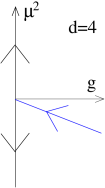
Restricting to the plane of couplings parameterised by $\mu^{2}$ and $g_{4}$ , we see that (if we neglect the interactions) the RG flow near the origin is very different when $d>4$ and $d<4$ . These are shown in the two figures. In the former case, we need to tune only $\mu^{2}\sim T-T_{c}$ if we want to hit the fixed point; the other couplings will take care of themselves. In contrast, when $d<4$ both of these couplings are relevant. This means that we would need to tune both to zero if we want to hit the Gaussian fixed point.

We can tally this with our discussion in Section 3.2. The fact that the scaling dimension $\Delta_{\phi}$ coincides with the naive engineering dimension $[\phi]$ immediately tells us that $\eta=0$ . Meanwhile, the scaling of $\mu^{2}\sim t$ is given by $\Delta_{t}=[g_{2}]=2$ , which tells us that $\nu=1/2$ . From this we can use (3.77) - (3.80) to extract the remaining critical exponents. These agree with mean field for $d=4$ , but not for $d\leq 4$ . (We will address the situation in $d>4$ in Section 3.3.2.)

It is no coincidence that this behaviour switches at $d=4$ , which we previously identified as the upper critical dimension. In an experiment, one can always change $\mu^{2}$ by varying the temperature. However, one may not have control over the $\phi^{4}$ couplings which typically correspond to some complicated microscopic property of the system. If $\phi^{4}$ is irrelevant, we don’t care: the system will drive itself to the Gaussian fixed point. In contrast, if $\phi^{4}$ is relevant the system will drive itself elsewhere. This is why we don’t measure mean field values for the critical exponents: these are the critical exponents of the Gaussian fixed point.

The coupling for $\phi^{6}$ scales as

\displaystyle g_{6}(\zeta)=\zeta^{6-2d}g_{0,6}

This is irrelevant in $d>3$ , relevant in $d<3$ and, naively, marginal in $d=3$ .

Note that in dimension $d=2$ all of the couplings $g_{n}\phi^{n}$ are relevant.

So far, this all looks rather trivial. However, things become much more interesting at other fixed points. For example, around most fixed points $\Delta_{\phi^{n}}\neq n\Delta\phi$ . Indeed, around most fixed points neither $\phi$ nor $\phi^{n}$ will have well defined scaling dimension; instead those operators to which one can assign a scaling dimension consist of some complicated linear combination of the $\phi^{n}$ . We will start to understand this better in Section 3.4.

The Meaning of Mean Field

Figure 26: The phase diagram of the Ising model.

The phase diagram of the liquid-gas system. — Figure 26: The phase diagram of the Ising model.

The meaning of the phrase “mean field theory” has evolved as these lectures have progressed. We started in Section 1.1.2 by introducing mean field as a somewhat dodgy approximation to the partition function. Subsequently, we used the expression “mean field theory” to mean writing down a free energy $F[\phi]$ and focussing on the saddle point equations. This saddle point is a good approximation to the partition function only when the couplings are small; this is true only in the vicinity of the Gaussian fixed point. For this reason, using mean field theory is usually synonymous with working at the Gaussian fixed point, and ignoring the effect of operators like $\phi^{4}$ on fluctuations. (Of course, mean field still retains the $\phi^{4}$ term in the ordered phase, where it is needed to stabilise the potential.)

Interactions that Break ${\bf Z}_{2}$ Symmetry

Until now, we have have restricted ourselves to interactions $\phi^{n}$ with $n$ even, to zealously safeguard the ${\bf Z}_{2}$ symmetry $\phi\rightarrow-\phi$ . One particularly nice aspect of RG is that if we restrict ourselves to a class of free energies that obey a certain symmetry, then we will remain in that class under RG. We’ll see examples of this in Section 3.4.

However, suppose that we sit outside of this class and turn on interactions $\phi^{n}$ with $n$ odd. The leading order effect is the magnetic field $B\phi$ that we included in our original Ising model. This is always a relevant interaction. This means that if we want to hit the critical point, we must tune this to zero.

It may be more natural to tune $B=0$ in some systems that others. For example, a magnet in the Ising class automatically has $B=0$ unless you choose to submit it to a background magnetic field. This means that it’s easy to hit the critical point: just heat up a magnetic and it will exhibit a second order phase transition.

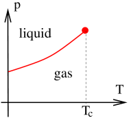
In contrast, in the liquid gas system, setting “ $B=0$ ” is less natural. Unlike in the Ising model, there is no ${\bf Z}_{2}$ symmetry manifest in the microscopic physics of gases. Instead, it is an emergent symmetry which relates the density of liquid and gas states at the phase transition. Correspondingly, if we simply take a liquid and heat it up then we’re most likely to encounter a first order transition, or no transition at all. If we want to hit the critical point, we must now tune the two relevant operators: temperature $\mu^{2}$ and pressure, which corresponds to the linear term with coefficient $B$ .

In both situations above we really need to tune two relevant couplings to zero to hit the critical point. Of these, one is even under ${\bf Z}_{2}$ and one is odd under ${\bf Z}_{2}$ . Doing this will allow us to hit a fixed point with two relevant deformations, one even one odd. This is the Gaussian fixed point in $d>4$ and is something else (to be described below) in $d<4$ .

What about higher order interactions $\phi^{n}$ with $n$ odd. If we have to tune $\phi$ , do we not also need to tune $\phi^{3}$ ? It turns out that that the $\phi^{3}$ interaction is redundant. If you have a free energy with no ${\bf Z}_{2}$ symmetry, and all powers of $\phi^{n}$ , then you can always redefine your field as $\phi\rightarrow\phi+c$ for some constant $c$ . This freedom allows you to eliminate the $\phi^{3}$ term. Note that if your free energy enjoys the ${\bf Z}_{2}$ symmetry $\phi\rightarrow-\phi$ then it prohibits you from making this shift.

3.3.2 Dangerously Irrelevant

We’ve learned that the $\phi^{4}$ interaction is irrelevant for $d\geq 4$ , and so one can hit the Gaussian fixed point by tuning just one parameter: $\mu^{2}=0$ .

However, there’s one tricky issue that we haven’t yet explained: the mean field exponents agree with the scaling analysis of Section 3.2 only when $d=4$ . Comparing the two results, we have

	$\alpha$	$\beta$	$\gamma$	$\delta$	$\eta$	$\nu$
MF	$\frac{4-d}{2}$	$\frac{1}{2}$	1	3	0	$\frac{1}{2}$
Scaling	$\frac{4-d}{2}$	$\frac{d-2}{4}$	1	$\frac{d+2}{d-2}$	0	$\frac{1}{2}$

where we’ve used the result (2.47), including quadratic fluctuations, for the mean field value of $\alpha$ . This agrees with the scaling analysis. However, for $d>4$ , the exponents $\beta$ and $\delta$ differ. It turns out that the results from Landau mean field are correct, and those from the scaling analysis are wrong. Why?

To understand this, let’s recall our scaling argument from Section 3.2. We set $B=0$ and focus on the critical exponent $\beta$ . The magnetisation scales with the temperature $t=|T-T_{c}|/T_{c}$ as

\displaystyle m\sim t^{\beta}

Here $m$ is identified with the scalar field $\phi$ . Scaling analysis gives $\Delta_{\phi}=\beta\Delta_{t}$ . But both mean field and scaling analysis agree that $\Delta_{t}=1/\nu=2$ and $\Delta_{\phi}=(d-2)/2$ , and this gives $\beta=(d-2)/4$ , rather than the mean field result $\beta=1/2$ .

However, we were a little quick in the scaling analysis because we neglected the quartic coupling $g_{4}$ . Mean field really told us (1.31),

\displaystyle m_{0}\sim\left(\frac{t}{g_{4}}\right)^{1/2}

But both $t$ and $g_{4}$ scale under RG flow. The scaling dimension of $g_{4}$ is $\Delta_{g_{4}}=4-d$ and now the mean field result, with $\beta=1/2$ is fully compatible with scaling.

There’s a more general lesson to take from this. It is tempting, when doing RG, to think that we can just neglect the irrelevant operators because their coefficients flow to zero as we approach the infra-red. However, sometimes we will be interesting in quantities – such as the magnetisation above – which have the irrelevant coupling constants sitting in the denominator. In this case, one cannot just blindly ignore these irrelevant couplings as they affect the scaling analysis. When this happens, the irrelevant coupling is referred to as dangerously irrelevant.

3.3.3 An Aside: The Emergence of Rotational Symmetry

This is a good point to revisit an issue that we previously swept under the rug. We started our discussion with a lattice model, but very quickly moved to the continuum, field theory. Along the way we stated, without proof, that we expect the long distance physics to enjoy rotational invariance and we restricted our attention to field theories with this property. Why are we allowed to do this?

To make the discussion concrete, consider a square lattice in $d=2$ dimensions. This has a discrete ${\bf Z}_{4}$ rotational symmetry, together with a ${\bf Z}_{2}$ reflection symmetry. These combine together into the dihedral group $D_{8}$ .

Our field theory description will respect the $D_{8}$ symmetry of the underlying lattice model, together with the ${\bf Z}_{2}$ symmetry $\phi\rightarrow-\phi$ which ensures that fields come in pairs. But this would appear to be much less powerful than the full $O(2)$ continuous rotation and reflection symmetry. Have we cheated?

Let’s see what kind of terms we might expect. First, there are some simple terms that are prohibited by the dihedral symmetry. For example a lone term $(\partial_{1}\phi)^{2}$ would break the $x_{1}\rightarrow x_{2}$ discrete rotational symmetry and so would not appear in the free energy. Similarly, a term $\phi\partial_{1}\phi$ breaks the $x_{1}\rightarrow-x_{1}$ symmetry. (On top of this, it is also a total derivative and so doesn’t contribute to the free energy.) The lowest dimension term that includes derivatives and is compatible with the discrete symmetry is

\displaystyle{\cal O}_{2}\sim(\partial_{1}\phi)^{2}+(\partial_{2}\phi)^{2}

But this term happens to be invariant under the full, continuous $O(2)$ rotational symmetry. We should keep going. The first term that preserves $D_{8}$ , but not $SO(2)$ , is

\displaystyle{\cal O}_{4}\sim\phi\partial_{1}^{4}\phi+\phi\partial_{2}^{4}\phi

There is no reason not to add such terms to the free energy and, in general, we expect that these will be present in any field theoretic description that accurately describes the microscopic physics. However, this operator has dimension $\Delta_{{\cal O}_{4}}=d+2$ and so is irrelevant. This means that it gets washed away by the renormalisation group, and the long wavelength physics is invariant under the full $O(2)$ symmetry. We say that the continuous rotational symmetry is emergent. A similar argument holds for higher dimensions.

3.4 RG with Interactions

The previous section left two questions hanging. What happens to the renormalisation of the coupling $g_{4}$ in $d=4$ dimensions? And where does the flow of $g_{4}$ take us in $d<4$ dimensions? In this section we will answer the first of these. In Section 3.5 we will see that our analysis also contains the answer to the second.

We now repeat our RG procedure, but with a different starting point in theory space,

\displaystyle F[\phi]=\int d^{d}x\ \left[\frac{1}{2}\nabla\phi\cdot\nabla\phi+% \frac{1}{2}\mu_{0}^{2}\phi^{2}+g_{0}\phi^{4}\right]

The renormalisation group procedure tells us to split the Fourier modes of the field into long and short wavelengths,

\displaystyle\phi_{{\bf k}}=\phi_{{\bf k}}^{-}+\phi_{{\bf k}}^{+}

(3.89)

and write the free energy as

\displaystyle F[\phi]=F_{0}[\phi^{-}]+F_{0}[\phi^{+}]+F_{I}[\phi^{-},\phi^{+}]

where we take $F_{0}[\phi]$ to coincide with the quadratic terms (3.83), and the interaction terms are

\displaystyle F_{I}[\phi]=\int d^{d}x\ g_{0}\phi^{4}

Note that we’ve chosen to include, for example, $(\phi^{-})^{4}$ in the interaction terms rather than $F_{0}$ . This is a matter of convention.

The effective free energy for $\phi_{{\bf k}}^{-}$ , defined in (3.68), is given by

\displaystyle e^{-F^{\prime}[\phi^{-}]}=e^{-F_{0}[\phi_{{\bf k}}^{-}]}\int{% \cal D}\phi_{{\bf k}}^{+}\ e^{-F_{0}[\phi_{{\bf k}}^{+}]}e^{-F_{I}[\phi_{{\bf k% }}^{-},\phi_{{\bf k}}^{+}]}

There is a nice interpretation of this functional integral $\int{\cal D}\phi_{{\bf k}}^{+}$ . We can think of it as computing the expectation value of $e^{-F_{I}[\phi_{{\bf k}}^{-},\phi_{{\bf k}}^{+}]}$ , treating $\phi_{{\bf k}}^{+}$ as the random variable with Gaussian distribution $e^{-F_{0}[\phi_{{\bf k}}^{+}]}$ . In other words, we can write this as

\displaystyle e^{-F^{\prime}[\phi^{-}]}=e^{-F_{0}[\phi_{{\bf k}}^{-}]}\,\left<% e^{-F_{I}[\phi_{{\bf k}}^{-},\phi_{{\bf k}}^{+}]}\right>_{+}

where the subscript on $\langle\cdot\rangle_{+}$ is there to remind us that we are averaging over the $\phi_{{\bf k}}^{+}$ modes only. We take the definition of the path integral to be suitably normalised so that $\langle 1\rangle_{+}=1$ . Taking the log of both sides,

\displaystyle F^{\prime}[\phi^{-}]=F_{0}[\phi_{{\bf k}}^{-}]-\log\left<e^{-F_{% I}[\phi_{{\bf k}}^{-},\phi_{{\bf k}}^{+}]}\right>_{+}

(3.90)

Our task is to compute this.

We can’t do this functional integral exactly. Instead, we resort to perturbation theory. We assume that $g_{0}$ is suitably small, and expand. (The dimensionless small parameter is $g_{0}\mu_{0}^{d-4}$ .) We first Taylor expand the exponential,

\displaystyle\log\left<e^{-F_{I}[\phi_{{\bf k}}^{-},\phi_{{\bf k}}^{+}]}\right% >_{+}=\log\left<1-F_{I}+\frac{1}{2}F_{I}^{2}+\ldots\right>_{+}

and we then Taylor expand $\log(1+x)$ , to get

\displaystyle\log\left<e^{-F_{I}[\phi_{{\bf k}}^{-},\phi_{{\bf k}}^{+}]}\right% >_{+}=-\left<F_{I}\right>_{+}+\frac{1}{2}\left[\left<F_{I}^{2}\right>_{+}-% \left<F_{I}\right>_{+}^{2}\right]+\ldots

(3.91)

where, in general, the $n^{\rm th}$ term is $(-1)^{n}\times n^{\rm th}$ cumulant of $F_{I}$ . This also follows from the same kind of manipulations that we did at the beginning of Section 2.2. We will deal with each of terms above in turn.

3.4.1 Order $g_{0}$

At leading order in $g_{0}$ , we need to compute $\left<F_{I}[\phi_{{\bf k}}^{-},\phi_{{\bf k}}^{+}]\right>_{+}$ . The first order of business is to expand the interaction terms (3.90) in Fourier modes. We have

\displaystyle F_{I}[\phi_{{\bf k}}^{-},\phi_{{\bf k}}^{+}]=g_{0}\int\prod_{i=1% }^{4}\frac{d^{d}k_{i}}{(2\pi)^{d}}\times\left(\mbox{terms with $\phi$}\right)% \times(2\pi)^{d}\delta^{d}(\sum_{i}{\bf k}_{i})

There are five different “terms with $\phi$ ”, most of which do not give anything interesting. These five terms are:

i)

$\phi^{-}_{{\bf k}_{1}}\phi^{-}_{{\bf k}_{2}}\phi^{-}_{{\bf k}_{3}}\phi^{-}_{{% \bf k}_{4}}$ : This term doesn’t include any $\phi_{{\bf k}}^{+}$ , the average is trivial. It carries over to give the term $g_{0}\int d^{d}x\ \phi^{-\,4}$ in the effective free energy.
ii)

$4\phi^{-}_{{\bf k}_{1}}\phi^{-}_{{\bf k}_{2}}\phi^{-}_{{\bf k}_{3}}\phi^{+}_{{% \bf k}_{4}}$ : This term has just a single $\phi_{{\bf k}}^{+}$ and so vanishes when averaged over the Gaussian ensemble.
iii)

$6\phi^{-}_{{\bf k}_{1}}\phi^{-}_{{\bf k}_{2}}\phi^{+}_{{\bf k}_{3}}\phi^{+}_{{% \bf k}_{4}}$ : This term is interesting. We will look at it more closely below. For now, note that the factor of 6 comes from the different choices of momentum labels.
iv)

$4\phi^{-}_{{\bf k}_{1}}\phi^{+}_{{\bf k}_{2}}\phi^{+}_{{\bf k}_{3}}\phi^{+}_{{% \bf k}_{4}}$ : This term is cubic in $\phi_{{\bf k}}^{+}$ and, like any term with an odd number of insertions, vanishes when averaged over the Gaussian ensemble.
v)

$\phi^{+}_{{\bf k}_{1}}\phi^{+}_{{\bf k}_{2}}\phi^{+}_{{\bf k}_{3}}\phi^{+}_{{% \bf k}_{4}}$ : This term doesn’t include any $\phi_{{\bf k}}^{-}$ , it simply gives constant to the free energy. It will not be important here.

We learn that we need to compute just a single term,

\displaystyle\left<F_{I}\right>_{+}=6g_{0}\int\prod_{i=1}^{4}\frac{d^{d}k_{i}}% {(2\pi)^{d}}\,\phi^{-}_{{\bf k}_{1}}\phi^{-}_{{\bf k}_{2}}\times\left<\phi^{+}% _{{\bf k}_{3}}\phi^{+}_{{\bf k}_{4}}\right>_{+}\times(2\pi)^{d}\delta^{d}(\sum% _{i}{\bf k}_{i})

(3.92)

But this is the same kind of correlation function that we computed in Section 2.2: it is given by

\displaystyle\left<\phi^{+}_{{\bf k}}\phi^{+}_{{\bf k}^{\prime}}\right>_{+}=(2% \pi)^{d}\delta^{d}({\bf k}+{\bf k}^{\prime})\,G_{0}(k)\ \ \ {\rm with}\ \ \ \ % G_{0}(k)=\frac{1}{k^{2}+\mu_{0}^{2}}

(3.93)

After playing around with the delta-functions, and relabelling momentum variables, we’re left with our first correction to the free energy,

\displaystyle\left<F_{I}\right>_{+}=6g_{0}\int_{0}^{\Lambda/\zeta}\frac{d^{d}k% }{(2\pi)^{d}}\,\phi^{-}_{{\bf k}}\phi^{-}_{-{\bf k}}\ \int_{\Lambda/\zeta}^{% \Lambda}\frac{d^{d}q}{(2\pi)^{d}}\frac{1}{q^{2}+\mu_{0}^{2}}

where the limits on the $\int dq$ integral reflect the fact that we’ve only integrated out the short wavelength modes, whose momenta lie within this band. We see that, at order $g_{0}$ , we get a correction only to the quadratic term whose coefficient becomes

\displaystyle\mu_{0}^{2}\rightarrow\mu^{\prime\,2}=\mu_{0}^{2}+12g_{0}\int_{% \Lambda/\zeta}^{\Lambda}\frac{d^{d}q}{(2\pi)^{d}}\frac{1}{q^{2}+\mu_{0}^{2}}

(3.94)

Finally, we should enact the rescaling steps of the renormalisation group. This takes the same form as before (3.84),

\displaystyle{\bf k}^{\prime}=\zeta{\bf k}\ \ \ {\rm and}\ \ \ \phi^{\prime}_{% {\bf k}}=\zeta^{-w}\phi_{{\bf k}/\zeta}^{-}\ \ \ {\rm with}\ \ \ w=\frac{d+2}{2}

This gives the same scaling of the parameters that we saw in Section 3.3. We have

\displaystyle\mu^{2}(\zeta)=\zeta^{2}\left(\mu_{0}^{2}+12g_{0}\int_{\Lambda/% \zeta}^{\Lambda}\frac{d^{d}q}{(2\pi)^{d}}\frac{1}{q^{2}+\mu_{0}^{2}}\right)\ % \ \ {\rm and}\ \ \ g(\zeta)=\zeta^{4-d}g_{0}

(3.95)

The upshot of this calculation is that turning on a $\phi^{4}$ coupling will give rise to a quadratic $\phi^{2}$ coupling under RG flow. This is typical of these kinds of calculations: couplings of one type will induce others.

The coefficient of the $\phi^{2}$ term is particularly important for our story, since the critical point is defined to be the place where this vanishes. We see that it’s not so easy to make this happen. You can’t simply set $\mu^{2}_{0}=0$ at some high scale and expect to hit criticality. Indeed, the result (3.95) tells us that, at long wavelengths, the “natural” value is $\mu^{2}\sim g_{0}\Lambda^{d-2}$ , which is typically large. If you want to hit the critical point, you must “fine tune” the original coefficient $\mu_{0}^{2}$ to cancel the new terms that are generated by RG flow.

You might think that this calculation answers the question of what happens to the theory in $d=4$ when we turn on $g\phi^{4}$ . It certainly tells us that turning on this coupling will induce the relevant coupling $\mu^{2}\phi^{2}$ and so take us away from the Gaussian fixed point. However, a closer look at (3.95) reveals that it’s possible to turn on a combination of $g_{0}$ and $\mu_{0}^{2}$ , so that $\mu^{2}(\zeta)$ remains zero. This combination is a marginal coupling. We learn that, at this order, there remains one relevant and one marginal deformation.

3.4.2 Order $g_{0}^{2}$

The corrections to the $\phi^{4}$ terms first arise at order $g_{0}^{2}$ . Here we have the contribution

\displaystyle F^{\prime}[\phi^{-}]\sim-\frac{1}{2}\left(\langle F_{I}^{2}% \rangle-\langle F_{I}\rangle^{2}\right)

(3.96)

Expanding out $\langle F_{I}^{2}\rangle$ , we find 256 different terms. We will see how to organise them shortly, but for now we make a few comments before focussing on the term of interest.

Some of the terms in $\langle F_{I}^{2}\rangle$ will result in corrections that cannot be written as a local free energy, but are instead of the form $\left(\int d^{d}xf(\phi^{-})\right)^{2}$ for some $f(\phi)$ . These terms will be cancelled by the $\langle F_{I}\rangle^{2}$ terms. This is a general phenomena which you can learn more about in the lectures on Quantum Field Theory. In terms of Feynman diagrams, which we will introduce below, these kind of terms correspond to disconnected diagrams.

The terms that we care about in $\langle F_{I}^{2}\rangle$ are those which can be written as local corrections to the free energy. Of immediate interest for us are a subset of terms in $F_{I}^{2}\sim\int d^{d}x\,d^{d}y\ \phi^{4}({\bf x})\,\phi^{4}({\bf y})$ , given by

	$\displaystyle\frac{1}{2}\langle F_{I}^{2}\rangle_{+}\sim\frac{1}{2}{4\choose 2% }^{2}g_{0}^{2}\int_{0}^{\Lambda/\zeta}$		$\displaystyle\!\!\prod_{i=1}^{4}\left[\frac{d^{d}k_{i}}{(2\pi)^{d}}\ \phi_{{{% \bf k}}_{i}}^{-}\right]\int_{\Lambda/\zeta}^{\Lambda}\prod_{j=1}^{4}\left[% \frac{d^{d}q_{j}}{(2\pi)^{d}}\right]\ \langle\phi^{+}_{{\bf q}_{1}}\phi^{+}_{{% \bf q}_{2}}\phi^{+}_{{\bf q}_{3}}\phi^{+}_{{\bf q}_{4}}\rangle_{+}$
			$\displaystyle\times\ \ (2\pi)^{2d}\delta^{d}({\bf k}_{1}+{\bf k}_{2}+{\bf q}_{% 1}+{\bf q}_{2})\delta^{d}({\bf k}_{3}+{\bf k}_{4}+{\bf q}_{3}+{\bf q}_{4})$

Let’s explain what’s going on here. Each $\phi({\bf x})$ is decomposed into Fourier modes $\phi^{-}$ and $\phi^{+}$ . The same is true for each $\phi({\bf y})$ . In the above term, we have chosen two $\phi^{-}$ out of the $\phi^{4}({\bf x})$ and two $\phi^{-}$ out of the $\phi^{4}({\bf y})$ ; the remaining terms are $\phi^{+}$ . Each combinatoric factor ${4\choose 2}=6$ out front reflects the choice of picking two $\phi^{-}$ from $\phi^{4}$ . Meanwhile, the two delta functions come from doing the $\int d^{d}x$ and $\int d^{d}y$ integrals respectively. Matching the momenta in the arguments of the delta functions to the $\phi^{\pm}$ tells us that we’ve picked two $\phi^{-}$ from the $\phi^{4}({\bf x})$ and two $\phi^{-}$ from $\phi^{4}({\bf y})$ (as opposed to, say, all four from $\phi^{4}({\bf y})$ ).

To proceed, we need to compute the four-point function $\langle\phi^{+}_{{\bf q}_{1}}\phi^{+}_{{\bf q}_{2}}\phi^{+}_{{\bf q}_{3}}\phi^% {+}_{{\bf q}_{4}}\rangle_{+}$ . To do this we need a result known as Wick’s theorem.

Wick’s Theorem

As we proceed in our perturbative expansion, the integrals start to blossom. From the form of the expansion (3.91), we can see that the integrand will involve expectation values of the form $\langle\phi^{+}_{{\bf k}_{1}}\ldots\phi^{+}_{{\bf k}_{l}}\rangle_{+}$ . There is a simple way to compute expectation values of this type in Gaussian ensembles. This follows from:

Lemma: Consider $n$ variables $\phi_{a}$ drawn from a Gaussian ensemble. This means that, for any function $f({\phi})$ , the expectation value is

\displaystyle\left<f(\phi)\right>=\frac{1}{{\cal N}}\int_{-\infty}^{\infty}d^{% n}\phi\ f(\phi)\,e^{-\frac{1}{2}\phi\cdot G^{-1}\phi}

for some invertible $n\times n$ matrix $G$ . The normalisation factor is ${\cal N}={\rm det}^{1/2}(2\pi G)$ and ensures that $\langle 1\rangle=1$ . The following identity then holds:

\displaystyle\left<e^{B_{a}\phi_{a}}\right>=e^{\frac{1}{2}B_{a}\left<\phi_{a}% \phi_{b}\right>B_{b}}

(3.98)

for any constant $B^{a}$ .

Proof: This is straightforward to show since we can just evaluate both sides

	$\displaystyle\left<e^{B_{a}\phi_{a}}\right>$	$\displaystyle=$	$\displaystyle\frac{1}{\cal N}\int_{-\infty}^{\infty}d^{n}y\ e^{-\frac{1}{2}% \phi\cdot G^{-1}\phi+B\cdot\phi}$
		$\displaystyle=$	$\displaystyle\frac{1}{\cal N}\int_{-\infty}^{\infty}d^{n}y\ e^{-\frac{1}{2}(% \phi-GB)\cdot G^{-1}(\phi-GB)}e^{\frac{1}{2}B\cdot GB}=e^{\frac{1}{2}B\cdot GB% }=e^{\frac{1}{2}B_{a}\left<\phi_{a}\phi_{b}\right>B_{b}}$

where, in the last step, we used the fact that $\langle\phi_{a}\phi_{b}\rangle=G_{ab}$ . $\Box$

The Taylor expansion of the identity (3.98) gives us the expressions that we want. The left-hand-side is

\displaystyle\left<e^{B_{a}\phi_{a}}\right>=1+B_{a}\langle\phi_{a}\rangle+% \frac{1}{2}B_{a}B_{b}\langle\phi_{a}\phi_{b}\rangle+\frac{1}{3!}B_{a}B_{b}B_{c% }\langle\phi_{a}\phi_{b}\phi_{c}\rangle+\frac{1}{4!}B_{a}B_{b}B_{c}B_{d}% \langle\phi_{a}\phi_{b}\phi_{c}\phi_{d}\rangle+\ldots

Meanwhile, the right-hand-side is

\displaystyle e^{\frac{1}{2}B_{a}\left<\phi_{a}\phi_{b}\right>B_{b}}=1+\frac{1% }{2}B_{a}B_{b}\langle\phi_{a}\phi_{b}\rangle+\frac{1}{8}B_{a}B_{b}B_{c}B_{d}% \langle\phi_{a}\phi_{b}\rangle\langle\phi_{c}\phi_{d}\rangle+\ldots

Now we just match powers of $B_{a}$ on both sides. We immediately learn that

\displaystyle\langle\phi_{a_{1}}\ldots\phi_{a_{l}}\rangle=0\ \ \ \mbox{for $l$% odd}

Our real interest is in $l$ even. Here we have to be a little careful because multiplying by the string of $B$ ’s automatically symmetrises the products of $\langle\phi_{a}\phi_{b}\rangle$ over the $a=1,\ldots,n$ indices. So, for example, comparing the $B^{4}$ terms gives

\displaystyle\langle\phi_{a}\phi_{b}\phi_{c}\phi_{d}\rangle=\langle\phi_{a}% \phi_{b}\rangle\langle\phi_{c}\phi_{d}\rangle+\langle\phi_{a}\phi_{c}\rangle% \langle\phi_{b}\phi_{d}\rangle+\langle\phi_{a}\phi_{d}\rangle\langle\phi_{b}% \phi_{c}\rangle

(3.99)

It’s not hard to convince yourself that

\displaystyle\langle\phi_{a_{1}}\ldots\phi_{a_{2l}}\rangle=\langle\phi_{a_{1}}% \phi_{a_{2}}\rangle\ldots\langle\phi_{a_{2l-1}}\phi_{a_{2l}}\rangle+\ \mbox{symmetrised}

This leaves us with a sum over all pairwise contractions. This result is known as Wick’s theorem.

Back to the Free Energy

We can now apply Wick’s theorem to our free energy (3.4.2),

\displaystyle\langle\phi^{+}_{{\bf q}_{1}}\phi^{+}_{{\bf q}_{2}}\phi^{+}_{{\bf q% }_{3}}\phi^{+}_{{\bf q}_{4}}\rangle_{+}=\langle\phi^{+}_{{\bf q}_{1}}\phi^{+}_% {{\bf q}_{2}}\rangle_{+}\langle\phi^{+}_{{\bf q}_{3}}\phi^{+}_{{\bf q}_{4}}% \rangle_{+}+\langle\phi^{+}_{{\bf q}_{1}}\phi^{+}_{{\bf q}_{3}}\rangle_{+}% \langle\phi^{+}_{{\bf q}_{2}}\phi^{+}_{{\bf q}_{4}}\rangle_{+}+\langle\phi^{+}% _{{\bf q}_{1}}\phi^{+}_{{\bf q}_{4}}\rangle_{+}\langle\phi^{+}_{{\bf q}_{2}}% \phi^{+}_{{\bf q}_{3}}\rangle_{+}

Recall that each of these propagators comes with a delta function,

\displaystyle\langle\phi^{+}_{{\bf q}}\phi^{+}_{{\bf q}^{\prime}}\rangle_{+}=(% 2\pi)^{d}\delta^{d}({\bf q}+{\bf q}^{\prime})\,G_{0}(q)

The trick is to see how these new delta functions combine with the original delta functions in (3.4.2). There are two different structures that emerge. The first term, gives (ignoring factors of $2\pi$ for now)

	$\displaystyle\int\prod_{j=1}^{4}d^{d}q_{j}$		$\displaystyle\!\!\!\!\!\!\langle\phi^{+}_{{\bf q}_{1}}\phi^{+}_{{\bf q}_{2}}% \rangle_{+}\langle\phi^{+}_{{\bf q}_{3}}\phi^{+}_{{\bf q}_{4}}\rangle_{+}% \delta^{d}({\bf k}_{1}+{\bf k}_{2}+{\bf q}_{1}+{\bf q}_{2})\,\delta^{d}({\bf k% }_{3}+{\bf k}_{4}+{\bf q}_{3}+{\bf q}_{4})$		(3.100)
		$\displaystyle\sim$	$\displaystyle\int d^{d}q_{2}d^{d}q_{4}\ G_{0}(q_{2})G_{0}(q_{4})\,\delta^{d}({% \bf k}_{1}+{\bf k}_{2})\,\delta^{d}({\bf k}_{3}+{\bf k}_{4})$		(3.100)

We’re still left with two delta functions over the ${\bf k}$ variables. This means that when we go back to real space, this term does not become a local integral. Instead, if you follow it through, it becomes a double integral of the form $\left(\int d^{d}x\ \phi^{-}({\bf x})^{2}\right)^{2}$ . As we explained after (3.96), these terms are ultimately cancelled by corresponding terms in $\langle F_{I}\rangle^{2}$ . They are not what interests us.

Instead, we care about the second and third terms in the Wick expansion of $\langle\phi^{+}_{{\bf q}_{1}}\phi^{+}_{{\bf q}_{2}}\phi^{+}_{{\bf q}_{3}}\phi^% {+}_{{\bf q}_{4}}\rangle_{+}$ . Each of them gives a contribution of the form

$\displaystyle\int\prod_{j=1}^{4}d^{d}q_{j}$		$\displaystyle\!\!\!\!\!\!\langle\phi^{+}_{{\bf q}_{1}}\phi^{+}_{{\bf q}_{3}}% \rangle_{+}\langle\phi^{+}_{{\bf q}_{2}}\phi^{+}_{{\bf q}_{4}}\rangle_{+}% \delta^{d}({\bf k}_{1}+{\bf k}_{2}+{\bf q}_{1}+{\bf q}_{2})\,\delta^{d}({\bf k% }_{3}+{\bf k}_{4}+{\bf q}_{3}+{\bf q}_{4})$	(3.101)
	$\displaystyle\sim$	$\displaystyle\int d^{d}q_{1}d^{d}q_{2}\ G_{0}(q_{1})\,G_{0}(q_{2})\,\delta^{d}% ({\bf k}_{1}+{\bf k}_{2}+{\bf q}_{1}+{\bf q}_{2})\,\delta^{d}({\bf k}_{3}+{\bf k% }_{4}-{\bf q}_{1}-{\bf q}_{2})$
	$\displaystyle\sim$	$\displaystyle\int d^{d}q\ G_{0}(q)\,G_{0}(\|{\bf k}_{1}+{\bf k}_{2}+{\bf q}\|)\,% \delta^{d}({\bf k}_{1}+{\bf k}_{2}+{\bf k}_{3}+{\bf k}_{4})$

where, in going to the last line, we have done the integral $\int d^{d}q_{2}$ and relabelled $q_{1}=q$ . Now we have just a single delta function over ${\bf k}_{i}$ and, correspondingly, when we go back to real space this will give a local contribution to the free energy. Indeed, the terms (3.4.2) now become

\displaystyle\frac{1}{2}\langle F_{I}^{2}\rangle_{+}\sim{4\choose 2}^{2}g_{0}^% {2}\int_{0}^{\Lambda/\zeta}\prod_{i=1}^{4}\left[\frac{d^{d}k_{i}}{(2\pi)^{d}}% \ \phi_{{{\bf k}}_{i}}^{-}\right]f({\bf k}_{1}+{\bf k}_{2})\ (2\pi)^{d}\delta^% {d}(\sum_{i}{\bf k}_{i})

(3.102)

where the factor of $\frac{1}{2}$ in (3.4.2) has disappeared because we get two contributions from the Wick expansion, each of which gives the same contribution (3.101). The remaining integral over $\int d^{d}q$ is hidden in the function $f({\bf k})$ , which is given by

\displaystyle f({\bf k}_{1}+{\bf k}_{2})=\int_{\Lambda/\zeta}^{\Lambda}\frac{d% ^{d}q}{(2\pi)^{d}}\ \frac{1}{q^{2}+\mu_{0}^{2}}\frac{1}{({\bf k}_{1}+{\bf k}_{% 2}+{\bf q})^{2}+\mu_{0}^{2}}

(3.103)

This is not as complicated as it looks. We can write it as

\displaystyle f({\bf k}_{1}+{\bf k}_{2})=\int_{\Lambda/\zeta}^{\Lambda}\frac{d% ^{d}q}{(2\pi)^{d}}\frac{1}{(q^{2}+\mu_{0}^{2})^{2}}\left(1+{\cal O}({\bf k}_{1% },{\bf k}_{2})\right)

All the terms that depend on the external momenta ${\bf k}_{1}$ and ${\bf k}_{2}$ will generate terms in the free energy of the form $k^{2}(\phi^{-})^{4}\sim(\phi^{-})^{2}\nabla^{2}(\phi^{-})^{2}$ . These are irrelevant terms that will not be interesting for us other than to note that once we let loose the dogs of RG, we will no longer sit comfortably within some finite dimensional subspace of the coupling constants. Integrating out degrees of freedom generates all possible terms consistent with symmetries; flowing to the IR allows us to focus on the handful of relevant ones.

The contribution (3.102) to the free energy is what we want. Translating back to real space, we learn that the quadratic term gets corrections at this order. We have

\displaystyle g_{0}\rightarrow g_{0}^{\prime}=g_{0}-36g_{0}^{2}\int_{\Lambda/% \zeta}^{\Lambda}\frac{d^{d}q}{(2\pi)^{d}}\frac{1}{(q^{2}+\mu_{0}^{2})^{2}}

(3.104)

The minus sign in (3.104) is important. It can be traced to the minus sign in (3.96), and it determines the fate of the would-be marginal coupling $g\phi^{4}$ in $d=4$ dimensions. Recall that, in $d=4$ , there is no contribution to the running of $g(\zeta)$ from the second and third steps of RG. Here, the leading contribution comes from the first step and, as we see above, this causes $g(\zeta)$ to get smaller as $\zeta$ increases. This means that the theory in $d=4$ is similar in spirit to those in $d>4$ , with $\phi^{4}$ an irrelevant coupling.

However, in $d=4$ , the RG flow for $g$ happens much more slowly than other couplings. For this reason it is sometimes called marginally irrelevant, to highlight the fact that it only failed to be marginal when the perturbative corrections were taken into account. This is a general phenomenon: most couplings which naively appear marginal will end up becoming either marginally relevant or marginally irrelevant due to such corrections. In the vast majority of cases, the coupling turns out to be marginally irrelevant. However, there are a number of very important examples – the Kondo effect and non-Abelian gauge theories prominent among them – where a marginal coupling turns relevant. We’ll see such an example in Section 4.3.

Finally, just because $g$ is marginally irrelevant in $d=4$ does not mean that you can turn it on and expect to flow back to the Gaussian fixed point. As depicted in the diagram, the coupling mixes with $\mu^{2}$ . If you want to flow back to the Gaussian fixed point, you need to turn on a particular combination of $\mu_{0}^{2}$ and $g_{0}$ .

3.4.3 Feynman Diagrams

The calculation above needed some care. As we go to higher order terms in the expansion, the number of possibilities starts to blossom. Fortunately, there is a simple graphical formalism to keep track of what’s going on.

Suppose that we’re interested in a term in the expansion (3.91) of the form $g_{0}^{p}(\phi^{-})^{n}(\phi^{+})^{l}$ . This can be represented by one or more Feynman diagrams. Here is the game:

•

Each $\phi_{{\bf k}}^{-}$ is represented by an external, solid line.
•

Each $\phi_{{\bf k}}^{+}$ is represented by a dotted line.
•

The dotted lines are connected with each other to form internal loops. They are paired up in all possible ways, reflecting the pair contraction of Wick’s theorem. No dotted lines can be left hanging which means that the diagrams only make sense for $l$ even.
•

Each factor of $g_{0}$ is represented as a vertex at which four lines meet.
•

Each line has an attached momentum ${\bf k}$ which is conserved as we move around the diagram.

Each of these diagrams is really shorthand for an integral. The dictionary is as follows:

•

Each internal line corresponds to an insertion of the propagator $\left<\phi^{+}_{{\bf k}}\phi^{+}_{{\bf k}^{\prime}}\right>_{+}$ defined in (3.93)
•

For each internal loop, there is an integral $\int d^{d}q/(2\pi)^{d}$ .
•

Each vertex comes with a power of $g_{0}(2\pi)^{d}\delta^{d}(\sum_{i}{\bf k}_{i})$ where the delta function imposes momentum conservation, with the convention that all momenta are incoming.
•

There are a bunch of numerical coefficients known as symmetry factors.

This means that a term in the effective action of the form $g_{0}^{p}(\phi^{-})^{n}$ will correspond to a diagram with $n$ external lines and $p$ vertices. We can see what these diagrams look like for some of the terms that we’ve met so far. At order $g_{0}$ , the rules don’t allow us to draw diagrams with an odd number of $\phi_{{\bf k}}^{-}$ . The term $\phi^{-}_{{\bf k}_{1}}\phi^{-}_{{\bf k}_{2}}\phi^{-}_{{\bf k}_{3}}\phi^{-}_{{% \bf k}_{4}}$ in the expansion gives the trivial contribution to $\phi^{4}$ . In diagrams, it is

\displaystyle\raisebox{-19.35pt}{\epsfbox{sftfigs/phi1.eps}}=g\int d^{d}x\ (% \phi^{-})^{4}

(3.105)

Similarly, the $(\phi^{+})^{4}$ terms are $\phi^{+}_{{\bf k}_{1}}\phi^{+}_{{\bf k}_{2}}\phi^{+}_{{\bf k}_{3}}\phi^{+}_{{% \bf k}_{4}}\ \sim\ \raisebox{-5.59pt}{\epsfbox{sftfigs/phi3.eps}}$ , but because these are internal lines we should join them up to get a diagram that looks like .

The interesting term at order $g_{0}$ is $\phi^{-}_{{\bf k}_{1}}\phi^{-}_{{\bf k}_{2}}\phi^{+}_{{\bf q}}\phi^{+}_{-{\bf q}}$ , which includes both $\phi_{{\bf k}}^{-}$ and $\phi_{{\bf k}}^{+}$ . This was evaluated in (3.92). It is represented by the diagram

\displaystyle\raisebox{-19.35pt}{\epsfbox{sftfigs/phi2.eps}}=6g_{0}\int_{% \Lambda/\zeta}^{\Lambda}\frac{d^{d}q}{(2\pi)^{d}}\frac{1}{q^{2}+\mu_{0}^{2}}% \int d^{d}x\ (\phi^{-})^{2}

where the integral arises because the momentum ${\bf q}$ of the $\phi^{+}$ excitation running in the loop is not determined by momentum conservation of the external legs. Such corrections are said to arise from loop diagrams, as opposed to the tree diagrams of (3.105).

Finally, at order $g_{0}^{2}$ , the correction (3.102) to the $\phi^{4}$ coupling comes from the

\displaystyle\raisebox{-20.21pt}{\epsfbox{sftfigs/phioneloop.eps}}=36g_{0}^{2}% \int_{0}^{\Lambda/\zeta}

\displaystyle\!\!\prod_{i=1}^{4}\left[\frac{d^{d}k_{i}}{(2\pi)^{d}}\ \phi_{{{% \bf k}}_{i}}^{-}\right]f({\bf k}_{1}+{\bf k}_{2})\ (2\pi)^{d}\delta^{d}(\sum_{% i}{\bf k}_{i})

where the function $f({\bf k}_{1}+{\bf k}_{2})$ was given in (3.103) and contains two propagators associated to the $\phi^{+}$ fields running in the loop. Evaluating this leads to the correction (3.104), as well as a slew of higher derivative couplings.

Any graph that we can draw will appear somewhere in the expansion of $\log\langle e^{-F_{I}[\phi_{{\bf k}}^{-},\phi_{{\bf k}}^{+}]}\rangle_{+}$ given in (3.91). As we noted above, this is a cumulant expansion which has the rather nice graphical interpretation that only connected graphs appear in the expansion. For example, at order $g_{0}^{2}$ , the disconnected graph that appears in the expansion of $\langle F_{I}^{2}\rangle_{+}$ that looks like will be cancelled by the same disconnected graph appearing in $-\langle F_{I}\rangle^{2}_{+}$ .

In the language of quantum field theory, it’s tempting to view the lines in the Feynman diagrams as the worldlines of particles. There is no such interpretation in the present case: they’re simply useful.

More Diagrams

We can now also look at other diagrams and see what role they play. For example, you might be worried about the diagram . This is strictly vanishing, because the incoming momentum for lone $\phi^{-}$ leg is forced to be equal to the intermediate momentum for the $\phi^{+}$ propagator. Yet the momentum for $\phi^{-}$ and $\phi^{+}$ can never be equal .

There are, however, two further diagrams that we neglected which do have an interesting role to play. Both of these are two loop diagrams. They will not affect what we’re going to do later but, nonetheless, are worth highlighting. The first diagram is

\displaystyle\raisebox{-21.07pt}{\epsfbox{sftfigs/phionemore.eps}}\ =g_{0}^{2}% \int\frac{d^{d}k}{(2\pi)^{d}}\ \frac{1}{2}C(\Lambda)\phi_{{\bf k}}^{-}\phi^{-}% _{-{\bf k}}

for some $C(\Lambda)$ whose exact form will not be important. This gives rise to a shift in the quadratic term, so that (3.94) is replaced by

\displaystyle\mu_{0}^{2}\rightarrow\mu^{\prime\,2}=\mu_{0}^{2}+12g_{0}\int_{% \Lambda/\zeta}^{\Lambda}\frac{d^{d}q}{(2\pi)^{d}}\frac{1}{q^{2}+\mu_{0}^{2}}+g% _{0}^{2}C(\Lambda)

The second diagram is

\displaystyle\raisebox{-14.19pt}{\epsfbox{sftfigs/phieta.eps}}\ =g_{0}^{2}\int% \frac{d^{d}k}{(2\pi)^{d}}\ \frac{1}{2}A(k,\Lambda)\phi_{{\bf k}}^{-}\phi^{-}_{% -{\bf k}}

(3.106)

We’ve called the result of this diagram $A(k,\Lambda)$ ; again we won’t need its detailed form. Importantly, it is now a function of the external momentum $k$ . This means that it gives rise to two effects that are (in a technical sense) relevant. The first is that there is yet another renormalisation of $\mu^{2}$ , this time depending on $A(0,\Lambda)$ . The second is novel: upon Taylor expanding $A(k)=A(0)+\frac{1}{2}k^{2}A^{\prime\prime}(0)+\ldots$ , we get a contribution to the the gradient term, which is now

\displaystyle F^{\prime}[\phi]=\int d^{d}x\ \frac{1}{2}\gamma^{\prime}\nabla% \phi\cdot\nabla\phi+\ldots\ \ \ \ {\rm with}\ \gamma^{\prime}=1-2g_{0}^{2}A^{% \prime\prime}(0,\Lambda)

This, in turn, means that we need a new rescaling of the field. To order $g_{0}^{2}$ , we can write this as

\displaystyle{\bf k}^{\prime}=\zeta{\bf k}\ \ \ {\rm and}\ \ \ \phi^{\prime}_{% {\bf k}}=\frac{\zeta^{-(d+2)/2}}{1-g_{0}^{2}A^{\prime\prime}(0,\Lambda)}\,\phi% _{{\bf k}/\zeta}^{-}

This last, additional step is known as field renormalisation. (Actually, that’s not completely true. It should be known as “field renormalisation”, but instead is known as “wavefunction renormalisation”. This a terrible name, one that betrays the long and deep confusion that permeated the origins of this subject. Even in the context of quantum field theory, this rescaling has nothing to do with wavefunctions. It is a rescaling of fields!)

Although we won’t compute this field renormalisation exactly, it is nonetheless important for this is what gives rise to the anomalous dimension of $\phi$ , and this was underlying the whole scaling analysis of Section 3.2.

3.4.4 Beta Functions

It is useful to write down equations which describe the flow of the coupling constants. These are first order differential equations which, for historic reasons are known as beta functions. It turns out to be convenient to parameterise the change in cut-off as

\displaystyle\Lambda^{\prime}=\frac{\Lambda}{\zeta}=\Lambda e^{-s}

The renormalisation group transformation described above tells us that each coupling changes with scale, $g_{n}=g_{n}(s)$ . The beta function is defined as

\displaystyle\frac{dg_{n}}{ds}=\beta_{n}(g_{n})

Note that $s$ increases as we flow towards the IR. This means that a positive beta function tells us that $g_{n}$ gets stronger in the IR, while a negative beta function means that $g_{n}$ gets weaker in the IR. (As an aside: this is the opposite to how beta functions are sometimes defined in quantum field theory, where one parameterises the flow in terms of energy rather than length.)

Before we jump straight in, it’s useful to take a step backwards and build up the beta functions. Let’s go back to our original scaling analysis around the Gaussian fixed point (3.88), where the running of the couplings is given by $g_{n}(s)=e^{(d-nd/2+n)s}g_{0,n}$ . The beta functions are

\displaystyle\frac{dg_{n}}{ds}=\left(d-\frac{1}{2}nd+n\right)g_{n}

(3.107)

Notice that, at this leading order, there’s no mixing between different couplings: turning on one coupling $g_{n}$ does not induce another to flow. As we saw above, this state of affairs no longer holds when we include interactions.

We now focus on the two most important couplings, $\mu_{0}^{2}$ and $g_{0}$ . At order $g_{0}$ , the RG equations are given by (3.95); the additional correction at order $g_{0}^{2}$ , given in (3.104), means that these get replaced by

\displaystyle\mu^{2}(\zeta)=\zeta^{2}\left(\mu_{0}^{2}+ag_{0}\right)\ \ \ {\rm and% }\ \ \ g(\zeta)=\zeta^{4-d}(g_{0}-bg_{0}^{2})

(3.108)

where

\displaystyle a=12\int_{\Lambda/\zeta}^{\Lambda}\frac{d^{d}q}{(2\pi)^{d}}\frac% {1}{q^{2}+\mu_{0}^{2}}\ \ \ {\rm and}\ \ \ b=36\int_{\Lambda/\zeta}^{\Lambda}% \frac{d^{d}q}{(2\pi)^{d}}\frac{1}{(q^{2}+\mu_{0}^{2})^{2}}

Note that we have kept our original scaling dimensions in (3.108); the corrections in scaling due to the diagram (3.106) will be subleading and not needed in what follows.

When we differentiate $\mu^{2}(\zeta)$ and $g(\zeta)$ to derive the beta functions, we will get two terms: the first is (3.107) and comes from the scaling; the second comes from the corrections, given by the integrals $a$ and $b$ . Differentiating these integrals is particularly easy. For small $s$ , we we write

\displaystyle\int^{\Lambda}_{\Lambda e^{-s}}dq\ f(q)\approx[\Lambda-\Lambda e^% {-s}]f(\Lambda)\approx\Lambda f(\Lambda)s\ \ \ \Rightarrow\ \ \ \frac{d}{ds}% \int_{\Lambda e^{-s}}^{\Lambda}dq\ f(q)=\Lambda f(\Lambda)

Let’s restrict to $d=4$ dimensions. The beta function equations are

\displaystyle\frac{d\mu^{2}}{ds}=2\mu^{2}+\dfrac{3g}{2\pi^{2}}\frac{\Lambda^{4% }}{\Lambda^{2}+\mu^{2}}\ \ \ {\rm and}\ \ \ \dfrac{dg}{ds}=-\frac{9}{2\pi^{2}}% \frac{\Lambda^{4}}{(\Lambda^{2}+\mu^{2})^{2}}g^{2}

(3.109)

These don’t (yet) contain any new physics, but it’s worth reiterating what information we can extract from these equations.

First, the beta function for $\mu^{2}$ has two terms; the first term comes from the second and third steps in RG (scaling), while the second comes from the first step in RG (integrating out). Meanwhile, the beta function for $g$ has only a single term. There is no term linear in $g$ because it was marginal under scaling, but it does receive a contribution when we integrate out the high momentum modes at order $g^{2}$ . This contribution is negative, which tells us the coupling is marginally irrelevant. (A repeat of the warning above: this is the opposite convention to quantum field theory where one flows in decreasing energy, rather than increasing length, which means that a marginally irrelevant interaction is usually said to have a positive beta function. )

3.4.5 Again, the Analogy with Quantum Field Theory

The calculations above are very similar to the kind of loop integrals that you do in quantum field theory in $d=3+1$ dimensions. There are, however, some philosophical differences between the approaches.

In statistical mechanics, the field $\phi({{\bf x}})$ is, by construction, a coarse grained object: at the microscopic level, it dissolves into constituent parts, whether spins or atoms or something else. This has the practical advantage that we have no expectation that the statistical field theory will describe physics on arbitrarily short distance scales. In contrast, when we talk about quantum field theory in the context of high energy physics, it is tempting to think of the fields as “fundamental”, a basic building block of our Universe. We may then wish for the theory to make sense down to arbitrarily small distance scales.

This ambition leads to a subtly different viewpoint on renormalisation. In quantum field theory one must introduce a cut-off, as we have above, to render integrals finite. However, this cut-off is very often viewed as an artefact, one which we would ultimately like to get rid of and make sense of the theory as $\Lambda\rightarrow\infty$ . The trouble is that the renormalised quantities – things that we’ve called $\mu^{2}$ and $g$ – typically depend on this cut-off. We saw this, for example, in (3.108). Often this makes it tricky to take the limit $\Lambda\rightarrow\infty$ .

To avoid this problem, one makes the so-called bare couplings – things we’ve called $\mu_{0}^{2}$ and $g_{0}$ – depend on $\Lambda$ . This is not such a dumb thing to do; after all, these quantities were defined at the cut-off scale $\Lambda$ . The original game of renormalisation was to find a way to pick $\mu_{0}^{2}(\Lambda)$ and $g_{0}(\Lambda)$ such that all physical quantities remain finite as $\Lambda\rightarrow\infty$ . It is by no means obvious that this is possible. Theories which can be rendered finite in this way are said to be renormalisable.

The high-energy approach to renormalisation predates the statistical physics approach and is now considered rather old-fashioned. The idea that a theory needs to make sense up to arbitrarily high energy scales smacks of hubris. The right way to view renormalisation – whether in statistical mechanics or in high energy physics – is through the renormalisation group procedure that has been our main focus in this chapter, in which one integrates out short wavelength modes to leave an effective long-distance theory.

Nonetheless, the high-energy approach to renormalisation has its advantages. Once one goes beyond the calculations described above, things are substantially easier with a high-energy viewpoint. You will learn more about these issues in the lectures on Advanced Quantum Field Theory.

3.5 The Epsilon Expansion

We have learned that $\phi^{4}$ interaction is irrelevant for $d\geq 4$ and relevant for $d<4$ , sweeping us away from the Gaussian fixed point. But we seem to be no closer to figuring out where we end up. All we know is that we’re not in Kansas anymore.

The difficulty is that we’re limited in what we can calculate. We can’t do the path integral exactly in the presence of $\phi^{4}$ interactions, and are forced to work perturbatively in the coupling $g$ . Yet, as we have seen, in dimension $d<4$ the RG flow increases $g$ , taking us to a regime where perturbation theory is no longer valid.

Figure 29: The beta function for

g

when

d<4

. The arrows show the flow of

g

as we move towards the infra-red. The fixed point lies within the regime of perturbation theory when

d=4-\epsilon

Nonetheless, the calculations that we did above do contain information about where we might expect to end up. But to see it, we have to do something rather dramatic. We will consider our theories not in $d=4$ dimensions, but in

\displaystyle d=4-\epsilon

dimensions where $\epsilon$ is a small number, much less than 1. Clearly, this is an odd thing to do. You could view it as an act of wild creativity or, one of utter desperation. Probably it is a little bit of both. But, as we shall see, it will give us the insight we need to understand critical phenomena.

First, we should ask whether it makes sense to work in a non-integer dimension. The lattice models that we started with surely need to be defined in dimension $d\in{\bf Z}^{+}$ . Similarly, it was important for us that the free energy is local, meaning that it is written as an integral over space, and this too requires $d\in{\bf Z}^{+}$ . However, by the time we get to the beta function equations, it makes mathematical, if not physical, sense to relax this and work in arbitrary $d\in{\bf R}$ . We can read off these beta functions from the RG equations (3.108): they are

	$\displaystyle\frac{d\mu^{2}}{ds}$	$\displaystyle=$	$\displaystyle 2\mu^{2}+\frac{12\Omega_{d-1}}{(2\pi)^{d}}\frac{\Lambda^{4}}{% \Lambda^{2}+\mu^{2}}\tilde{g}+\ldots$
	$\displaystyle\frac{d\tilde{g}}{ds}$	$\displaystyle=$	$\displaystyle\epsilon\tilde{g}-\frac{36\Omega_{d-1}}{(2\pi)^{d}}\frac{\Lambda^% {4}}{(\Lambda^{2}+\mu^{2})^{2}}\tilde{g}^{2}+\ldots$

where $\Omega_{d-1}$ is the area of the sphere ${\bf S}^{d-1}$ . We’ve introduced the dimensionless coupling $\tilde{g}=\Lambda^{-\epsilon}g$ . Note that the beta function for $\tilde{g}$ now includes a term linear in $\tilde{g}$ arising from the scaling.

It can be checked that the two-loop diagrams we neglected contribute only at order $\epsilon^{2}$ . This means that it’s consistent to truncate to the beta functions above. We could use the general formula for the area of a sphere, $\Omega_{d-1}={2\pi^{d/2}}/{\Gamma(d/2)}$ , but this will give corrections of order $\epsilon^{2}$ , so instead we simply use $\Omega_{3}=2\pi^{2}$ . Similar comments apply to $(2\pi)^{d}$ . We’re left with

	$\displaystyle\frac{d\mu^{2}}{ds}$	$\displaystyle\approx$	$\displaystyle 2\mu^{2}+\frac{3}{2\pi^{2}}\frac{\Lambda^{4}}{\Lambda^{2}+\mu^{2% }}\tilde{g}$
	$\displaystyle\frac{d\tilde{g}}{ds}$	$\displaystyle\approx$	$\displaystyle\epsilon\tilde{g}-\frac{9}{2\pi^{2}}\frac{\Lambda^{4}}{(\Lambda^{% 2}+\mu^{2})^{2}}\tilde{g}^{2}$

The novelty of these beta functions is that they have two fixed points. There is the Gaussian fixed point $\mu^{2}=\tilde{g}=0$ that we discussed before. And there is a new fixed point,

\displaystyle\mu^{2}_{\star}=-\frac{3}{4\pi^{2}}\frac{\Lambda^{4}}{\Lambda^{2}% +\mu_{\star}^{2}}\tilde{g}_{\star}\ \ \ {\rm and}\ \ \ \tilde{g}_{\star}=\frac% {2\pi^{2}}{9}\frac{(\Lambda^{2}+\mu_{\star}^{2})^{2}}{\Lambda^{4}}\epsilon

Since we’re working to leading order in $\epsilon$ , the solution is

\displaystyle\mu^{2}_{\star}=-\frac{3}{4\pi^{2}}\Lambda^{2}\tilde{g}_{\star}=-% \frac{1}{6}\Lambda^{2}\epsilon\ \ \ {\rm and}\ \ \ \tilde{g}_{\star}=\frac{2% \pi^{2}}{9}\epsilon

This is the Wilson-Fisher fixed point. Importantly, when $\epsilon$ is small then the fixed point $\tilde{g}_{\star}$ is also small, so our calculation is self-consistent (although, since we are in a fractional dimension, arguably unphysical!).

3.5.1 The Wilson-Fisher Fixed Point

To understand the flows in the vicinity of the new fixed point, we write $\mu^{2}=\mu_{\star}^{2}+\delta\mu^{2}$ and $\tilde{g}=\tilde{g}_{\star}+\delta\tilde{g}$ . Linearising the beta functions, we find

\displaystyle\frac{d}{ds}\left(\begin{array}[]{c}\delta\mu^{2}\\ \delta\tilde{g}\end{array}\right)=\left(\begin{array}[]{cc}2-\epsilon/3&\ % \frac{3}{2\pi^{2}}\Lambda^{2}\left(1+\frac{\epsilon}{6}\right)\\ 0&-\epsilon\end{array}\right)\left(\begin{array}[]{c}\delta\mu^{2}\\ \delta\tilde{g}\end{array}\right)

where, as with all our other calculations, the entries in the matrix hold only up to ${\cal O}(\epsilon^{2})$ .

The eigenvalues of a triangular matrix coincide with the diagonal entries. We see that this fixed point has one positive and one negative eigenvalue,

\displaystyle\Delta_{t}=2-\frac{\epsilon}{3}+{\cal O}(\epsilon^{2})\ \ \ {\rm and% }\ \ \ \Delta_{g}=-\epsilon+{\cal O}(\epsilon^{2})

In other words, the Wilson-Fisher fixed point has one relevant direction and one irrelevant. The flows are shown in the figure.

We see that the epsilon expansion provides us with a global picture of the RG flows in $d<4$ dimensions. One can check that all other couplings are also irrelevant at the Wilson-Fisher fixed point. Crucially, the fixed point sits at small $g$ where our perturbative analysis is valid.

Now suppose that we increase $\epsilon$ . The Wilson-Fisher fixed point moves to higher $g$ , and our perturbative approach breaks down. Nonetheless, it is not unreasonable to suppose that the qualitative picture of the flows remains the same. Indeed, this is thought to happen. Because the Wilson-Fisher fixed point has just a single relevant operator, it means that we will generically end up there if we we’re willing to tune just a single parameter, namely $T\rightarrow T_{c}$ .

It is now a simple matter to compute the critical exponents in the epsilon expansion. Recall from Section 3.2 that these are related to the scaling dimensions of various terms. The relevant direction away from the Wilson-Fisher fixed point is temperature, $t=|T-T_{c}|/T_{c}$ . Its dimension is determined by the way it scales as we approach the critical point, $t\rightarrow\zeta^{\Delta_{t}}t=e^{s\Delta_{t}}t$ . But this is precisely the eigenvalue $\Delta_{t}$ that we just computed.

The critical exponent $\nu$ , defined by $\xi\sim t^{-\nu}$ , is then given by (3.76)

\displaystyle\nu=\frac{1}{\Delta_{t}}=\frac{1}{2}+\frac{\epsilon}{12}+{\cal O}% (\epsilon^{2})

We can then use the hyperscaling relation $\alpha=2-d\nu$ , given in (3.77), to compute the critical exponent for the heat capacity

\displaystyle c\sim t^{-\alpha}\ \ \ {\rm with}\ \ \ \alpha=\frac{\epsilon}{6}% +{\cal O}(\epsilon^{2})

To compute the other critical exponents, we need to evaluate the anomalous dimension $\eta$ . As we mentioned briefly above, this is related to the diagram and turns out to be $\eta=\epsilon^{2}/6$ , which is higher order in the expansion. We then have, from (3.74),

\displaystyle\Delta_{\phi}\approx\frac{d-2}{2}=1-\frac{\epsilon}{2}

Equations (3.78), (3.79) and (3.80) then give

\displaystyle\beta\approx\frac{1}{2}-\frac{\epsilon}{6}\ \ \ ,\ \ \ \gamma% \approx 1+\frac{\epsilon}{6}\ \ \ ,\ \ \ \delta\approx 3+\epsilon

where all expressions hold up to corrections of order ${\cal O}(\epsilon^{2})$ .

Of course, our real interest lies in the system at $d=3$ , or $\epsilon=1$ . It would be in poor taste to simply plug in $\epsilon=1$ . But I know that you’re curious. Here’s what we get:

	$\alpha$	$\beta$	$\gamma$	$\delta$	$\eta$	$\nu$
MF	0	$\frac{1}{2}$	1	3	0	$\frac{1}{2}$
$\epsilon=1$	0.17	$0.33$	$1.17$	4	$0$	0.58
$d=3$	0.1101	0.3264	1.2371	4.7898	0.0363	0.6300

Our answers are embarrassingly close to the correct values given the dishonest method we used to get there. One can, however, make this approach more respectable. The $\epsilon$ expansion has been carried out to order ${\cal O}(\epsilon^{5})$ . It is not a convergent series. Nonetheless, sophisticated resummation techniques can be used to make sense of it, and the resulting expressions give a fairly accurate account of the critical exponents.

The real power of the epsilon expansion, however, is more qualitative than quantitative; it usually – but not always – gives a reliable view of the structure of RG flows.

3.5.2 What Happens in $d=2$ ?

We have not yet discussed much about what happens in $d=2$ dimensions. Here the story is somewhat richer. The first hint of this can be seen in a simple analysis of the Gaussian fixed point, which shows that

\displaystyle\Delta_{\phi}=[\phi]=0

This means that the Gaussian fixed point has an infinite number of relevant deformations since $\phi^{n}$ , for each $n$ , is relevant.

It turns out that, in contrast to $d=3$ , there are actually an infinite number of fixed points in $d=2$ . Roughly speaking, the $n^{\rm th}$ fixed point can be reached from the Gaussian fixed point by turning on

\displaystyle F[\phi]=\int d^{2}x\ \frac{1}{2}(\nabla\phi)^{2}+g_{2(n+1)}\phi^% {2(n+1)}

Of course, as we’ve seen above, the RG flow is not quite so simple. When we turn on the coupling $g_{2(n+1)}\phi^{2(n+1)}$ we will generate all other terms, including $\phi^{2}$ and $\phi^{4}$ and so on. To reach the $n^{\rm th}$ fixed point, we should tune all such terms to zero as we flow towards the infra-red.

One can show that the $n^{\rm th}$ fixed point has $n$ relevant operators: schematically, these can be thought of as $\phi^{2},\phi^{4},\ldots,\phi^{2n}$ although, as above, there will be mixing between these. By turning on the least relevant operator, one can flow from the $n^{\rm th}$ fixed point to the $(n-1)^{\rm th}$ fixed point.

The results above are not derived using the $\epsilon=4-d$ expansion which, unsurprisingly, is not much use in $d=2$ . Instead, they rely on something new which we will briefly describe in Section 3.6.

3.5.3 A History of Renormalisation

“After about a month of work [at General Atomic Corp] I was ordered to write up my results, as a result of which I swore to myself that I would choose a subject for research where it would take at least five years before I had anything worth writing about. Elementary particle theory seemed to offer the best prospects of meeting this criterion.”

Kenneth Wilson

Renormalisation first entered physics in the context of quantum field theory, with the need to make sense of the UV divergences that arise in quantum electrodynamics. The theory, developed by Schwinger, Feynman, Tomonaga, Dyson and others, amounts to finding a consistent way to subtract one infinity from another, leaving behind a finite answer. This method yields excellent agreement with experiment but is, in the words of Feynman, a “dippy process”, in which the infinities are not so much understood as swept under a very large rug.

The first hint of something deeper – and the first hint of a (semi)-group action – was seen in the work of Gell-Mann and Low in 1954. They realised that one could define an effective charge of the electron, $e(\mu)$ where $\mu$ denotes the energy scale at which the experiment takes place. This interpolates between the physical charge, as $\mu\rightarrow 0$ , and the so called bare charge at high energies.

Meanwhile, throughout the 50s and 60s, a rather different community of physicists were struggling to understand second order phase transitions. It had long been known that Landau theory fails at critical points, but it was far from clear how to make progress, and the results that we’ve described in this course took several decades to uncover. In Kings College London, a group led by Cyril Domb stressed the importance of focussing on critical exponents; at Cornell University, Benjamin Widom showed that the relationships between critical exponents could be derived by invoking a scale invariance, albeit with little understanding of where such scale invariance came from; and at the University of Illinois, Leo Kadanoff introduced the idea of “blocking” in lattice models, a real-space renormalisation group in which one worked with successively coarser lattice models.

While many people contributed to these developments, the big picture, linking ideas from particle physics, statistical physics and condensed matter physics, is due mostly to…

Kenneth Wilson: 1936-2013

Ken Wilson received his PhD in 1961, working with Murray Gell-Mann on an assortment of topics in particle physics that fed his interest in the renormalisation group. He went on to spend much of the 1960s confused, scrabbling to understand the physics of scale, first in quantum field theory and later in the context of critical phenomena. He wrote very few papers in this time, but his reputation was strong enough to land him postdocs at Harvard and CERN and later even tenure at Cornell. (Some career advice for students: the strategy of being a genius and not writing anything rarely leads to such success.)

The floodgates opened in 1971 when Wilson set out his grand vision of the renormalisation group and, with his colleague Michael Fisher, suggested the epsilon expansion as a perturbative method to compute critical exponents in a paper charmingly titled “Critical Exponents in 3.99 Dimensions”. Wilson used these methods to solve the “Kondo problem” in which an isolated spin, sitting in a bath of mobile electrons, exhibits asymptotic freedom, and he was among the first to understand the importance of numerical approaches to solve statistical and quantum field theories, pioneering the subject of lattice gauge theory. In 1982 he was awarded the Nobel prize for his contributions to critical phenomena.

3.6 Looking Forwards: Conformal Symmetry

There are many questions that we have not yet answered? How do we know the critical exponents in $d=2$ exactly? How do we know that there are an infinite number of fixed points in $d=2$ ? Why are the critical exponents in $d=2$ rational numbers while, in $d=3$ they have no known closed form? How are we able to compute the $d=3$ critical exponents to 5 significant figures?

The answers to all these questions can be found in the emergence of a rich mathematical structure at the critical point. As we’ve seen throughout these lectures, the basic story of RG ensures that physics at the critical point is invariant under scale transformations

\displaystyle{\bf x}\rightarrow\lambda{\bf x}

(3.110)

More surprising is the fact that the physics is invariant under a larger class of symmetries, known as conformal transformations. These transformation consist of any map

\displaystyle{\bf x}\rightarrow\tilde{{\bf x}}({\bf x})\ \ \ {\rm such\ that}% \ \ \ \frac{\partial{\tilde{x}^{i}}}{\partial{x^{k}}}\frac{\partial{\tilde{x}^% {j}}}{\partial{x^{l}}}\,\delta_{ij}=\phi({\bf x})\delta_{kl}

(3.111)

for some function $\phi({\bf x})$ . Such conformal transformations have the property that they preserve angles between lines.

The equation (3.111) has obvious solutions, such as translations and rotations, for which $\phi({\bf x})=1$ . Furthermore, it is simple to see that the scaling (3.110) falls into the class of conformal transformations, with $\phi({\bf x})=\lambda^{2}$ . However, it turns out that there is one further, less intuitive transformation that obeys this condition. This is known as the special conformal transformation and is given by

\displaystyle x^{\prime i}=\frac{x^{i}-({\bf x}\cdot{\bf x})a^{i}}{1-2({\bf x}% \cdot{\bf a})+({\bf a}\cdot{\bf a})({\bf x}\cdot{\bf x})}

(3.112)

parameterised by an arbitrary vector ${\bf a}$ .

The first question that we should ask is: why are theories at the fixed points invariant under the larger group of conformal transformations, rather than just scale transformations? The answer to this, which goes somewhat beyond this course, involves a deeper understanding of the nature of the RG flows and hinges, crucially, on being able to construct a quantity which decreases monotonically along the flow. This quantity is, unhelpfully, called $c$ in $d=2$ dimensions, $f$ in $d=3$ dimensions and $a$ in $d=4$ dimensions, and the fact that it decreases monotonically is referred to as the $c$ -theorem, $f$ -theorem and $a$ -theorem respectively. Using this machinery, it is then possible to prove that scale invariance implies conformal invariance. (The proof is more clearcut in $d=2$ ; it relies on some extra assumptions in higher $d$ , and there is a general feeling that there is more to understand here.)

The existence of an extra symmetry (3.112) brings a newfound power to the study of fixed points. The $d$ translational symmetries, $\frac{1}{2}d(d-1)$ rotational symmetries, $d$ special conformal symmetries and single scale transformation combine to form the conformal group, which can be shown to be isomorphic to $SO(d+1,1)$ . All fields and, in particular, all correlation functions must fall into representations of this group, a fact which restricts their form. In recent years, our understanding of these representations has allowed new precision in the computation of critical exponents in $d=3$ dimensions. This programme goes by the name of the conformal bootstrap.

Conformal Symmetry in $d=2$

In $d=2$ dimensions, conformal symmetry turns out to be particularly powerful. The group of finite conformal transformations follows the pattern in higher dimensions, and is $SO(3,1)\cong SL(2,{\bf C})$ . However, something rather special happens if you look at infinitesimal transformations where one finds that many many more are allowed. In fact, there are an infinite number. This means that there is a powerful, infinite dimensional algebra, known as the Virasoro algebra, underlying conformal theories in $d=2$ dimensions. This places much stronger constraints on these fixed points, ultimately rendering many of them solvable without resorting to perturbation theory. This is the reason why the critical exponents are rational numbers which can be computed exactly. This is also what allows us to understand the structure of the infinite number of multi-critical fixed points described in Section 3.5.2.

Conformal field theory in $d=2$ dimensions is a vast subject which arises in many different areas of physics. Although originally developed to understand critical phenomena, it also plays an important role in the lectures on the Quantum Hall Effect and the lectures on String Theory, where you can find an introduction to the basics of the subject.